Your Backtest's Max Drawdown Is One Coin Flip; Here's The Number That Matters

Every systematic trader has stared at the same reassuring artifact: a backtest report showing a max drawdown of, say, 10%. It sits there next to the Sharpe ratio and the equity curve, and it feels like a fact. A boundary. Something you can size against.

It isn't. It's a coin flip that already landed.

The max drawdown in your backtest describes what happened to one specific ordering of your trades — the historical one. There is nothing structurally special about that ordering. Markets could have delivered the same set of winners and losers in a different sequence, and your drawdown would have been a different number entirely.

This distinction is not academic for anyone trading with a hard risk limit — a funded account, a prop firm evaluation, a fund mandate with a stop-out, or simply a personal rule about when to shut a strategy down. In those cases, drawdown isn't a psychological inconvenience. It's the line where the account ends. And with funded accounts now representing a fast-growing slice of US retail participation in futures and FX, a growing number of traders are sizing against limits they have never stress-tested.

What happens when you reshuffle the same trades

Consider a strategy with 200 trades, a 55% win rate and positive expectancy — the kind of profile that looks perfectly respectable on paper. Run the historical sequence and the max drawdown comes in at 10.4%.

Now take those exact same 200 trades. Same P&L. Same win rate. Same edge. Change nothing except the order in which they arrive, and run it 5,000 times.

The results are uncomfortable:

— Backtest (historical order): 10.4% max drawdown
— Median across 5,000 orderings: 12.3%
— 95th percentile: 19.1%
— Worst ordering: 31.6%

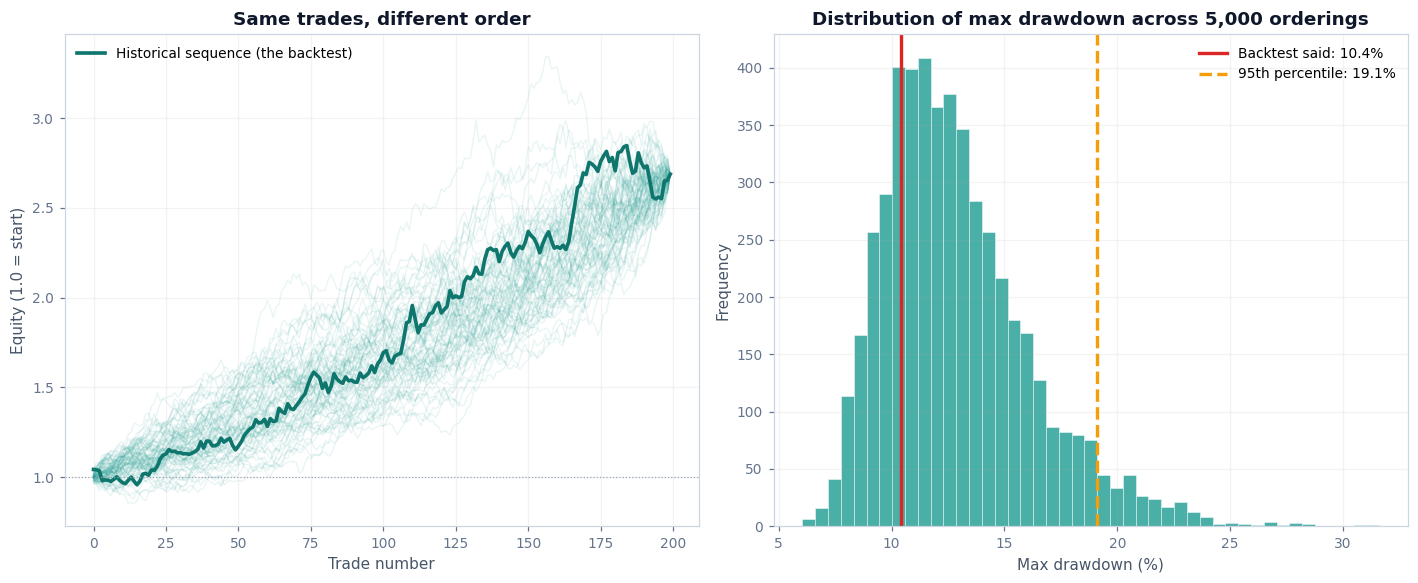
The strategy that "has a 10% drawdown" hits 19% in one out of twenty plausible futures, and 31% in the tail. Nothing about the edge changed. Only the sequence did.

A trader who sized this strategy against a 15% limit — comfortably above the backtest's 10.4% — would find that a meaningful share of alternative orderings breach it. The backtest didn't warn them, because the backtest only ever knew about one path.

Why losses cluster — and why simple reshuffling still understates the risk

The reshuffling exercise above assumes trades are independent, which flatters the strategy. In real markets they are not. Volatility is autocorrelated. Regimes persist. The conditions that produce a loss on Monday are frequently still there on Tuesday.

Losers arrive in bunches, and bunches are what end accounts.

A more honest simulation uses a block bootstrap: instead of resampling individual trades, resample contiguous blocks of them, preserving the local clustering that a naive shuffle destroys. Run that on the same strategy and the tail gets fatter still.

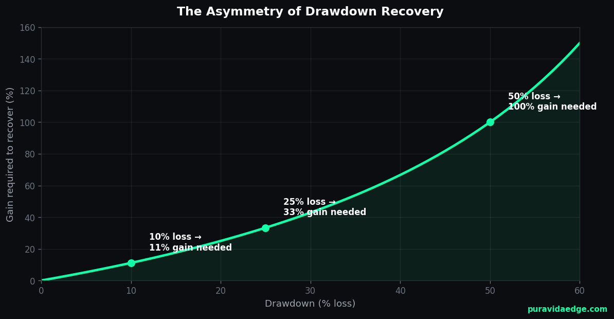
This matters most in instruments where volatility regimes are pronounced. Gold's average daily range can double between a quiet consolidation and a news-driven expansion, and index futures behave the same way around macro catalysts. A position size that was prudent in the first regime is reckless in the second — and the trader changed nothing. The market did. The arithmetic of getting back to even is worth internalizing here: a 20% loss needs a 25% gain, a 50% loss needs 100%. A simple drawdown recovery calculator makes that convexity obvious.

The number that actually matters

Once you have thousands of plausible orderings rather than one, the useful question stops being "what was my worst drawdown" and becomes:

What fraction of plausible paths breach my limit and end the account?

Call it the blow rate, or the probability of ruin. It converts a binary historical outcome ("we survived") into a probability ("we do not survive in 14% of plausible futures"). That is a number you can size against. A max drawdown from a single backtest is not. Readers who would rather run the distribution on their own trade history than take the argument on faith can do it with a Monte Carlo simulator ( that resamples paths and reports the breach rate directly.

The implication for position sizing is direct, and it is where most traders get it wrong. Doubling your size does not double your ruin risk — it tends to explode it, because drawdown scales roughly linearly with size while your distance to the limit does not. This convexity is why accounts that survive for years get destroyed in the month after a good run, when the trader "goes a bit bigger."

The disciplined version of sizing is not a rule of thumb. It is a constrained optimization: find the largest position size whose probability of breaching the limit stays under your tolerance. Anything larger is a bet that the sequence will be kind.

What simulation cannot fix

Honesty requires stating the limits. Resampling your history cannot invent a regime your history never contained; if your sample does not include a March 2020, no bootstrap will conjure one. Costs must already be embedded in the trade returns, or the entire exercise is fiction. And a curve-fit strategy will happily produce thousands of plausible futures for an edge that does not exist — simulation validates risk, not edge.

Used properly, it answers one question well, and it is the question that decides whether a trader is still trading next year: given that the edge is real, how likely am I to survive long enough to collect it?

The takeaway

A backtest tells you what happened once. It tells you nothing about how lucky you got in the telling. For any trader operating under a hard drawdown limit — and in an era of funded accounts and prop firm evaluations, that is a growing share of the retail market — the historical max drawdown is close to useless as a sizing input.

The distribution is the input. The single path is decoration.