In the debate over whether the establishment survey nonfarm payroll employment series is seriously overestimating recent (particularly Q2) employment, a reader querulously asks “So you’re saying the Philly Fed screwed up its analysis and we should ignore its work? That’s your view?”. Short answer to first question: No. Short answer to the second question: see below.

I take a lead from the Chow-Lin approach to interpolating/extrapolating via related series, and exploit the close relationship between the overall movement in the total covered employment series in the Quarterly Census of Employment and Wages (QCEW) and the nonfarm payroll employment series. Specifically, I follow this procedure:

1. Estimate the relationship between log NFP employment and log total covered employment, 2001-2019.
2. Use this relationship to predict NFP employment, both in-sample and out-of-sample
3. Verify that NFP employment is well predicted in out-of-sample period.
4. Interpretation

In order to allow the statistically challenged to understand the procedure (for instance, people who don’t know what a confidence interval is), show what I do in steps.

1. Estimation

I take data on NFP (FRED series PAYNSA) and QCEW total covered employment over the 2001-2022 period (QCEW data starts 2000M12). QCEW data are from a Census, and hence should not be subject to sampling error (QCEW data are used to benchmark update survey based estimates from the CES). Unfortunately, QCEW total covered employment are not reported in seasonally adjusted terms. Hence, I estimate the relationship between not-seasonally-adjusted series, in logs. These data are shown in Figure 1.

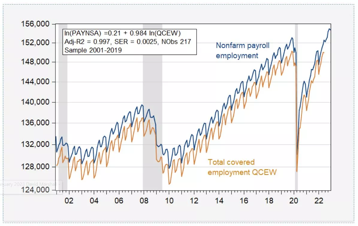
Figure 1: Nonfarm payroll employment (blue), total covered employment (tan), in 000’s, not seasonally adjusted. Nonfarm payroll series is FRED series PAYNSA; total covered series is BLS series ENUUS00010010. NBER defined peak-to-trough recession dates shaded gray. Source: BLS.

Note that the very high correlation. Running a regression (through 2019), the statistical fit is extremely good, with Adjusted R2 at 0.997.

The constant is pretty small, and the coefficient is near (but significantly different) from unity. Nonetheless, we are interested in prediction, so this point is not of concern. To guard against spurious correlation, I test for cointegration using the Johansen maximum likelihood method. I reject the null of zero cointegrating vectors (constant, no trend in cointegrating vector) at the 10%.

Why not estimate over the full sample, up to 2022? This yields a similarly good fit. However, a test using recursive residuals to evaluate structural breaks indicates that there’s a break at 2020M07, supporting the use of a sample that ends before the pandemic’s onset; this is shown in Figure 2.

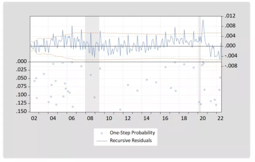
Figure 2: Recursive residuals from regression of log PAYNSA on log total covered QCEW employment. P-values on LHS scale.

2. Prediction

I use the equation estimated over 2001-19 to predict not seasonally adjusted NFP (PAYNSA). This is shown in Figure 2.

The fitted tracks the reported series fairly well. This is to be expected as the BLS series is benchmark updated using QCEW data.

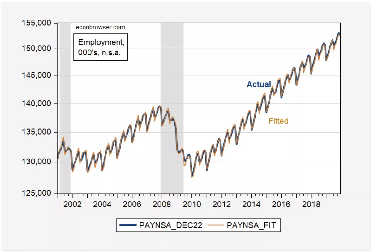
Figure 3: Reported nonfarm payroll employment, not seasonally adjusted (blue), fitted (tan). NBER defined peak-to-trough recession dates shaded gray. In-sample period shaded light green. Source: BLS, NBER, author’s calculations.

3. Out of sample fit

The equation used to fit the model is estimated over a period ending at 2019M12. That means 2020-2022M06 is the out of sample period that can be assessed (since QCEW data ends at 2022M06). These predictions are shown in Figure 4. Green denotes the in-sample period.

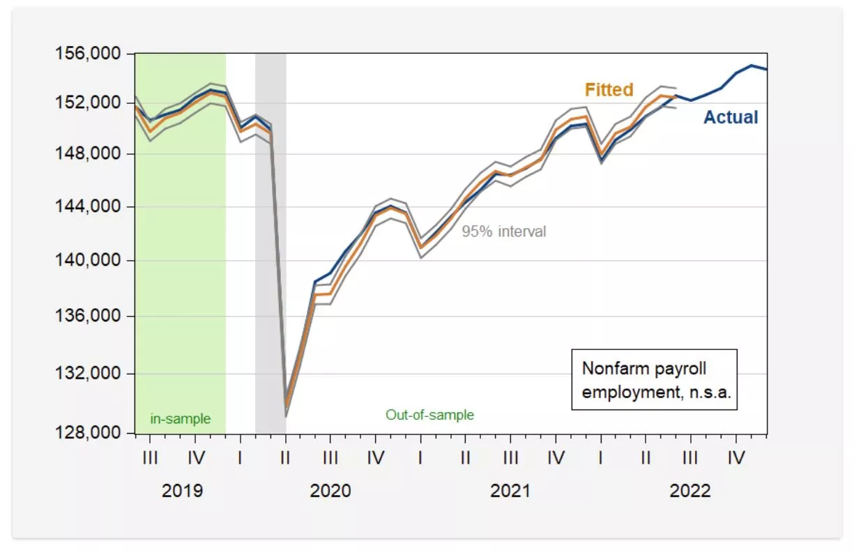
Figure 4: Reported nonfarm payroll employment, not seasonally adjusted (blue), fitted (tan),95% prediction interval (gray lines). NBER defined peak-to-trough recession dates shaded gray. In-sample period shaded light green. Source: BLS, NBER, author’s calculations.

In a period that spans the pandemic lockdown, the mean error is 50 thousand (remember NFP employment right now is about 153 million), maximum 1.9 million and minimum -866 thousand, standard deviation of 582 thousand.

4. Implications for the Debate

Interestingly, in the post-sample period, the model tends to underpredict reported employment for the most part. In other words, if the historical correlations hold, then the implied NFP should actually been higher than what was reported. As of March, the NFP number should’ve been higher by 291 thousand; and as of June, reported NFP was 155 thousand over what was predicted, so it is only in June that we have some evidence of over-estimation. While reported NFP was above predicted, it’s a much smaller number than nearly 1 million predicted by Philadelphia Fed.

These are not seasonally adjusted series. In order to convert my predicted values to those compatible with the usual referenced seasonally adjusted series (PAYEMS), I add the seasonal component as estimated by the BLS (PAYEMS-PAYNSA) to the predicted values shown in Figure 4. I show this implied series and the actual in Figure 5.

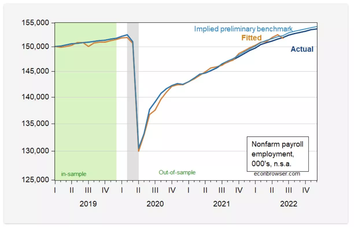
Figure 5: Reported nonfarm payroll employment, seasonally adjusted (blue), and fitted (tan), nonfarm payroll employment implied by preliminary benchmark revision (light blue), all in 000’s, s.a. NBER defined peak-to-trough recession dates shaded gray. In-sample period shaded light green. Implied benchmark revision series construction described in this post. Source: BLS, NBER, author’s calculations.

The fitted value of seasonally adjusted NFP is actually pretty close to the implied benchmark revision, calculated using the NFP numbers for March — updated using QCEW and other data, so this is not too surprising.

I show a detail of the most recent data, along with the BLS research series adjusting the civilian employment (household survey) series to the NFP concept (green line), as well as the Philadelphia Fed’s adjustment of QCEW data to fit NFP (red squares), in Figure 6.

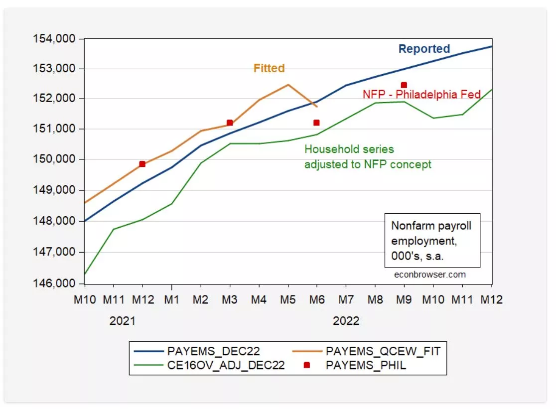
Figure 6: Reported nonfarm payroll employment, seasonally adjusted (blue), fitted (tan), BLS research series civilian employment adjusted to NFP concept (green), and Philadelphia Fed series (red squares), all in 000’s, s.a. NBER defined peak-to-trough recession dates shaded gray. Source: BLS, Philadelphia Fed, and author’s calculations.

My March figure for NFP closely matches the BLS series, both n.s.a. and s.a. (where I have used the BLS’s seasonal adjustments). My first observation is to note that this is a quick and dirty approach. It is not a wholesale defense of the benchmark un-revised series. Certainly there are reasons why the establishment series goes off track. In their “holistic” assessment, House and Pugliese/Wells Fargo highlighted the fact that the birth/death model could have been introducing too many new firms being created, thereby pushing up the NFP number. However, I am tracking using the QCEW, which is not subject to estimation error of this sort.

My second observation is that the fact that the Philadelphia Fed’s series implies a much lower NFP does not mean one or the other methodologies is wrong. It might mean that seasonal adjustment processes is distorting the results (either on the BLS side, or on the Philly Fed side, recalling how they are switching between geometric and additive errors), or the way the Philadelphia Fed reconciled state/sector data between the QCEW and the establishment survey imparted measurement error. Time will tell, in this case. I would never say ignore the Philadelphia Fed series; just consider alternative ways of looking at the data when evaluating the plausibility of the reported NFP series. Now, the civilian employment series consistently undershoots the official BLS series. Maybe it will turn out the household series is providing better signals about employment than the establishment and the Quarterly Census of Employment and Wages (remember it’s a census), but this is a little hard for me to understand, especially given the high variability of the household series.

More By This Author:

The Jobs Worker Gap In November
ADP Release, And The Flat Employment Growth In Q2 Thesis
Coincident Indicators Of Recession: VMT, Heavy Truck Sales, Sahm Rule