Now that the dust has (kind of) settled on exactly what is and is not in Gerald Friedman’s interpretation of the Sanders economic plan, I thought it useful to contrast the textbook (at least the one I use, Olivier Blanchard/David Johnson‘s) view of how a fiscal stimulus works, versus that in which a one-time spending increase yields a permanent increase in output, in a graphical format.

Textbook

In Figure 1, I depict steady state with output at the natural level/potential GDP, and price level at P16 (to denote price level in FY2016). I assume for simplicity that the output gap is zero; I myself believe it’s somewhat smaller, maybe around -2 to -3 percentage points of potential GDP.

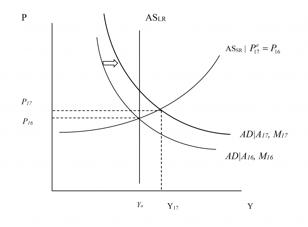
In FY2017, the AD curve is assumed to shift out due to an increase of government consumption and investment equal to about 0.8 percentage points of GDP; I assume this is a constant shift over the subsequent years, relative to where government spending was. The Fed accommodates somewhat, so part of the shift is due to increased money supply. The white arrow denotes the shift.

Notice that in the short output rises to FY18. Ignoring lags due to the spending multiplier taking time (the outside lag, in macro parlance), the AD curve stays where it is for the subsequent periods through FY2022.

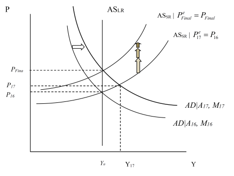
Over time, note that the aggregate supply curve adjusts upward. That’s because price expectations are adaptive (either because the underlying expectations process is adaptive, or because of nominal rigidities and nominal contracts that prevent instantaneous price adjustment), so the expected price level ratchets upward. As this happens, the real money supply shrinks, pushing up interest rates, so that investment falls. There’s a movement along the AD curve, and finally the AS curve stops shifting when the natural level of output is restored. In this sense, the model is one where the economy is self correcting.

In this textbook model, a fiscal stimulus delivers a temporary — and not necessarily persistent — increase in output above potential. This pattern matches the outcome discussed in this post.

Now, Jamie Galbraith has a plea to take seriously alternative models, and I am glad to do so. Doing so allows one to highlight what has to be assumed in order to “make it work”.

An Alternative View

It has been hard to glean exactly what assumptions were built into Gerald Friedman’s assessment, although I believe Romer and Romer have identified some of the key issues. It has been yet harder to understand what is involved in the various defenses of the Friedman assumption that multipliers apply to the growth of government spending, and not the level. As I interpret it, Friedman’s defense invokes (strong) hysteresis effects. How can permanent output effects, with minor impacts on inflation, be derived from such a view? Once again a graph can be helpful (it strikes me odd that nobody’s done this in the blogosphere — this is what I do for my macro class…).

First, assume we have a large negative output gap. Assume the aggregate supply curve is fairly flat (perfectly flat would do even better, but it’s not absolutely necessary). Or at least to begin with the AS curve is flat a position of a large negative output gap (Friedman cites -11%).

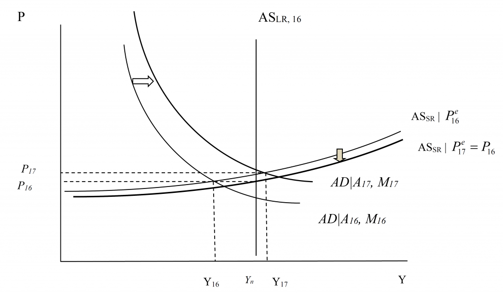
Then the increase in government spending that shifts out the AD curve in FY2017 results in a large increase in output with minimal added inflation. Now, what happens over time? In Figure 4, with the decline in the price level in FY2017 relative to FY2016, the short run AS curve shifts in.

More importantly, and critically, the increase in output in FY2017 (and the concurrent decrease in unemployment) results in a shift outward in thelong run AS curve. This is shown in Figure 4.

Note the short run AS curve shifts down in FY2017, so the resulting output is Y17. In FY2018, the long run AS curve shifts out so that the short run AS curve shifts out again in FY2018. The level of output again rises in FY2018. The process repeats itself in subsequent periods because higher output in a given period (recursively) results in a higher level of potential GDP.

This argument rationalizes the otherwise odd treatment of multipliers in the Friedman tabulation. To be fair, Friedman argues that potential GDP will also rise because of universal health care; however, the defense of the Friedman treatment of multipliers has hinged on hysteresis effects, so I’ve taken that literally.

Parting Thoughts

Obviously, each of these views grossly simplifies. In the textbook version, potential GDP is unaffected by recessions and slow growth. But it’s easily conceivable that the capital stock is lower than it would have been had economic conditions been buoyant and investment been higher (after all, net investment is the first derivative of the net capital stock…). Human capital too. The question is, how much.

So, in the Friedman worldview, how much does potential GDP respond to higher output due to a running a “high pressure” economy; how much institutional changes like universal health care, or infrastructure spending? And over what time frame do such effects take place?

Brad DeLong ponders some of these questions and provides some thoughts. I would like to think the AS curve is really, really flat, even past the level of potential GDP (i.e., no kinks in the AS curve), and I do believe to a certain extent (see this post). I believe that the payoff to infrastructure investment is quite high, and a no-brainer given current financing costs. But whether one could increase government consumption by nearly 8 percentage points of GDP and achieve highly persistent output increases, with only a one percentage point acceleration in inflation seems to me a question with an answer that is likely to be “no”. (For more on the plausibility of some of the implied elasticities, see Romer and Romer (2016).)