Two observations: (i) recessions do not necessarily coincide with negative output gaps (although they do seem to coincide with the beginning of periods of negative output gaps); and (ii) recoveries do not always coincide with positive output gaps. [This is an update of a 2008 post.]

This distinction can be illustrated by reference to the evolution of output in 2020, and forecasts.

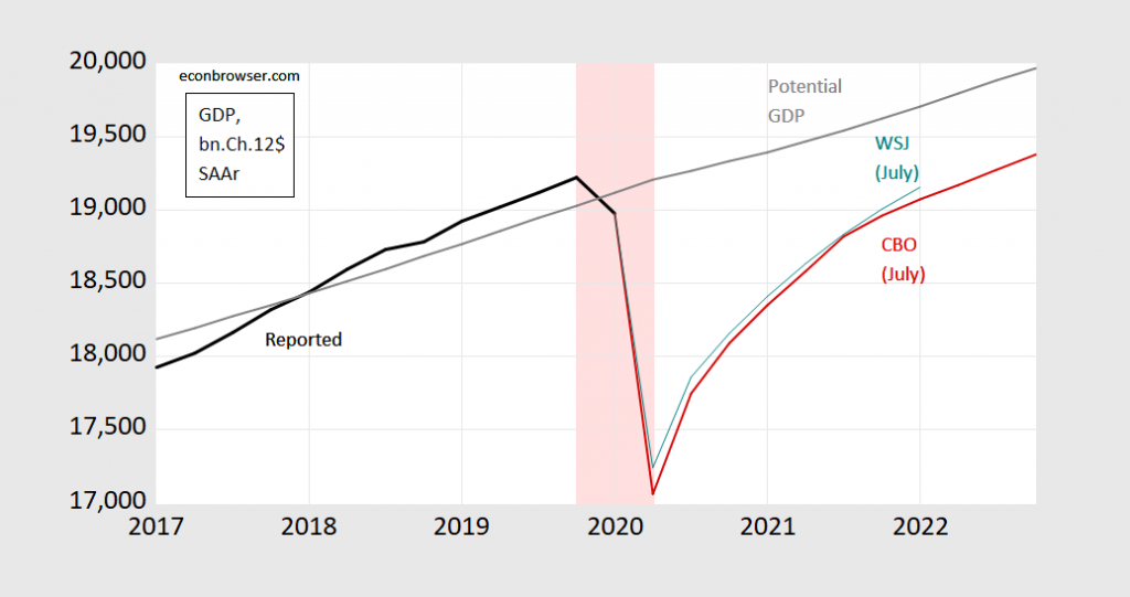
Figure 1: Real GDP (bn Ch.2012$, SAAR) (black line),potential GDP (gray line), CBO July projection (red line), and WSJ panel July survey mean (teal line). Hypothetical recession dates based upon NBER-defined peak date and 2020Q2 trough, shaded pink. Source: BEA, GDP 2020Q1 3rd release, and CBO, An Update of the Economic Outlook (July 2020), [data], NBER, and author’s calculations.

This difference is obvious when one thinks about it, given the NBER Business Cycle Dating Committee‘s definition of a recession (or “contraction”) as the following:

A recession is a significant decline in economic activity spread across the economy, lasting more than a few months, normally visible in real GDP, real income, employment, industrial production, and wholesale-retail sales. A recession begins just after the economy reaches a peak of activity and ends as the economy reaches its trough. Between trough and peak, the economy is in an expansion. Expansion is the normal state of the economy; most recessions are brief and they have been rare in recent decades.

That is a recession is the description of the first derivative of economic activity (broadly defined) taking on a negative value, while an output gap is a description of output relative to the output level consistent with the “normal” utilization of factors of production (also “full-employment”). For details of how CBO calculates potential GDP, see this document.

In the hypothetical recession dates shown above in pink, I use the NBER’s recently identified peak in 2019Q4 (for quarterly data, 2020M02 for monthly) as the start of the recession, and the lowest level of GDP in 2020Q2 as the “trough” (keeping in mind NBER does not use GDP as the sole indicator of economic activity; nor does the NBER use the oft-cited “2-consecutive quarter” rule of thumb). Then the recession is from 2019Q4 to 2020Q2, and expansion/recovery from 2020Q2 onward. In contrast, the negative output gap is obtains from 2020Q1 through the end of the sample in the graph. In fact, CBO projects that output will get within 1% of potential by 2027Q2. In other words, the technical (or NBER business cycle) definition of recovery doesn’t match the popular definition. [CEPR uses a slightly different methodology for the eurozone.]

There is of course a complication, one of particular relevance given the debate over a “W-shaped” recovery: if two local minima are sufficiently close together, does it make sense to count the short period between them as including an expansion? For instance, if Daniel Bachmann’s (Deloitte) July forecast (shown in the below figure) turns out to be accurate — and traces the path of the key indicators the NBER BCDC follows –, would that suggest two recessions or one?

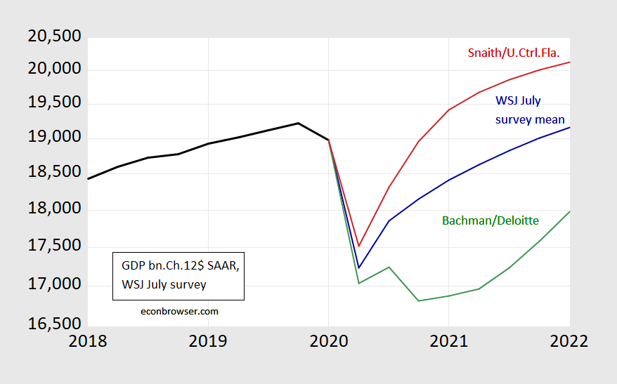
Figure 2: GDP in billions of Ch.2012$, SAAR, reported (black bold), WSJ July survey mean (blue), most “W” from Daniel Bachman at Deloitte (green), and one year most optimistic from Sean Snaith at University of Central Florida (red). Source: WSJ July survey, BEA, and author’s calculations.

Of course, the definition of a negative output gap — and determination of what magnitude — depends on an estimates of potential GDP. And this is variable that is not directly observable. CBO uses a production function approach, while time series methods are an alternative. Figure 3 depicts the July 2020 CBO estimate, and a time series method of extracting a trend.

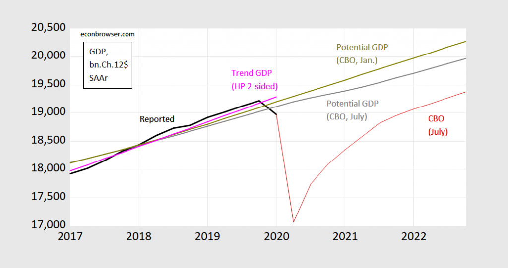
Figure 3: Real GDP (bn Ch.2012$, SAAR) (black line),potential GDP CBO estimate from July 2020 (gray line), from January 2020 (chartreuse line), HP filter (pink line), and CBO July 2020 projection (red line). Source: BEA, GDP 2020Q1 3rd release, and CBO, An Update of the Economic Outlook (July 2020), [data], Budget and Economic Outlook (January 2020), and author’s calculations.

The Hodrick-Prescott filter is a ubiquitous two-sided filter used in time series macroeconometrics and elsewhere. Essentially, the HP filter calculates a trend that minimizes the weighted sum of squared deviations from trend, and squared changes in the the growth rate of the trend. This weighting is controlled by a parameter which is usually set at 1600 for quarterly data. As a public service, I’ll note there are serious hazards associated with this filter, especially when trying to correlate various macro series that have been put through the same filter [1].

There is an additional problem (which is often ignored), namely that the HP filter is two-sided, so that running the filter up to the end point of data will tend to result in the trend being too close to the last data point (in our case, the output gap will be pulled to zero).

Alternative time series methods include band pass filters; the one most commonly used in the macroeconometric literature is the Baxter-King version. Band pass filters are called this because (in the frequency domain) they pass through any cyclical components within a particular frequency band, and elimates the others. In the time domain, this means fluctuations that are shorter or longer than a specific length are ignored. In the business cycle area, then, in order to use this filter, one would have to have a prior on how long a “typical” business cycle is. More on both the HP and BP filters can be found in Tim Cogley’s entry for the New Palgrave Dictionary of Economics [2]

In order to circumvent the two-sided filter aspect of the HP filter, one could do a standard fix, which is to use an ARIMA(1,1,1) on log GDP  to dynamically forecast out 12 quarters, and then apply the HP filter to this “extended” series. I could have done a similar procedure for the BP filter. Alternatively, one could use the Christiano and Fitzgerald (2003) one-sided asymmetric version of the band pass filter to estimate the trend series.

I implement these methods in this post, but for here, I’ll just note the difference between time series and production function approaches. And even different vintages of the CBO estimates vary, as additional information comes in. One might hope that the estimates don’t change too much between projections — but one can see from Figure 3 that in the case of the 2020 Covid-19 episode, there is a noticeable change.

[I skip issues related to data revisions which have implications on the use of real time vs. final revised data — see Orphanides and van Norden (2002) [pdf].]

Despite these complications, the distinction between the rate of change in economic output, and where output levels will gravitate to (and at what pace) is a useful one to keep in mind. [Or as I tell my students, just because you’re out of the recession and into a recovery doesn’t mean you’re not in a world of pain…]