Data released yesterday (CFS, SPGMI), through August.

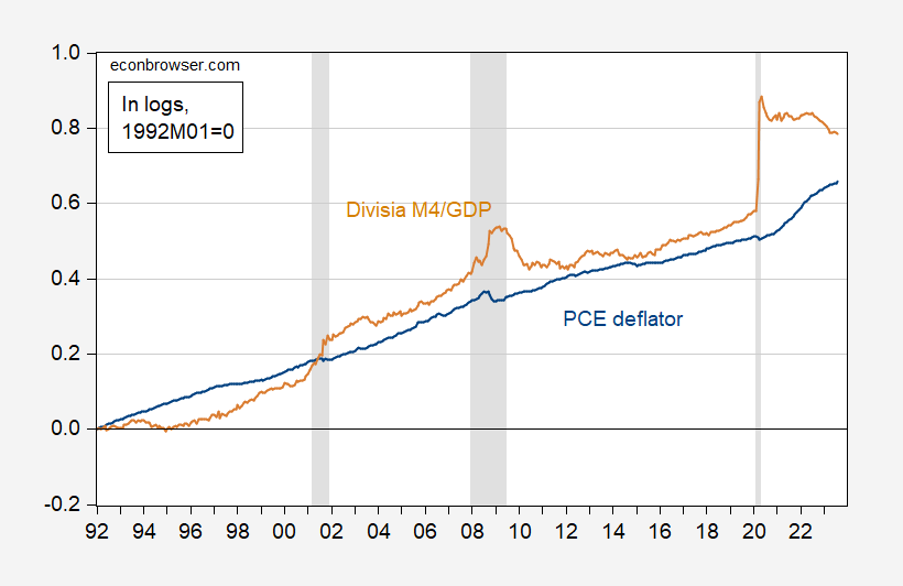
Figure 1: PCE deflator (blue), Divisia M4M divided by real GDP (tan), both in logs 1992M01=0. NBER defined peak-to-trough recession dates shaded gray. Source: BEA via FRED, Center for Financial Stability, SPGMI, NBER, and author’s calculations.

This plot is motivated by the Quantity Theory (here using broadest divisia index as one reader has demanded).

MV ≡ PQ

Where M is money, V is velocity, P is price level, Q is economic activity.

Assume V’ is constant; then:

MV’ = PQ

Take logs (where lowercase letters denote log values).

p = m + v’ – q 

During the 1992-2019 period (pre-pandemic), a multivariate cointegration test (constant in cointegrating vector, in VAR, but no deterministic trend in cointegrating vector, 4 lags of first differences) fails to reject the no cointegration null.

Instead of positing a long run trend velocity, one could posit a long run relationship between velocity and the interest rate (this is consistent with a stable long run money demand equation).

p = m + v(i) – q 

Where i is an interest rate. Add in the own-interest rate as calculated by Center for Financial Stability, and the same specification also fails.

If one adds 2020-2023M08 data, then cointegration is found at the 5% msl for the trend stationary velocity specification. It’s found at the 10% msl if interest rates are included. Unfortunately for this version of the quantity theory, the interest rate has the wrong signed (insofar as one believes in a money demand equation).

If one were forced to forecast on the basis of the (no-interest rate) quantity theory-based model, one would hit a small problem: besides the failure to find cointegration, the ratio of money to GDP seems to do the reversion to error correct — not the PCE deflator.

I estimated the single equation error correction model from 1992 to 2020.08 (which encompasses the big jump in Divisia M4), and forecast dynamically out of sample. This is what I get.

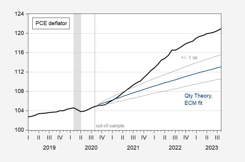
Figure 2: PCE deflator (black), and dynamic out-of-sample forecast (blue), +/- 1 standard error (gray lines). NBER defined peak-to-trough recession dates shaded gray. Source: BEA and author’s calculations.

While one could find other equally plausible parameter estimates, my point here is that the quantity theory taken literally does not necessarily fit the data well.

More By This Author: