Why You Should Never Use The Hodrick-Prescott Filter

A common problem in economics is that most of the variables we study have trends. Even the simplest statistics like the mean and variance aren’t meaningful descriptions of such variables. One popular approach is to remove the trend using the Hodrick-Prescott filter. I’ve just finished a new research paper highlighting the problems with this approach and suggesting what I believe is a better alternative.

The Hodrick-Prescott filter can be motivated as choosing a trend that is as close as possible to the observed series with a strong penalty for changing the trend too quickly. The typical value for the penalty parameter used for analyzing quarterly data is 1600. I show in my paper that for an observation at some date t near the middle of a large sample, the deviation from trend (denoted ct) that emerges from this procedure can be characterized as

Here 

 denotes the fourth difference– the change in the change in the change in the change. Maybe the growth rate (the first difference) has some trend, and maybe even the change in the growth rate (the second difference) has a trend too, but by the time we get to a fourth difference we’ve presumably taken all the trends out. All the other terms in the above expression put a lot of smoothness back in, but without any trends.

Is this a sensible procedure to apply to economic time series? The leading case we should consider is a random walk, which is a series for which the first difference (the change in the variable) is completely unpredictable. As I note in the paper [slightly rephrased]:

Simple economic theory suggests that variables such as stock prices (Fama, 1965), futures prices (Samuelson, 1965), long-term interest rates (Sargent, 1976; Pesando, 1979), oil prices (Hamilton, 2009), consumption spending (Hall, 1978), inflation, tax rates, and money supply growth rates (Mankiw, 1987) should all behave like random walks. To be sure, hundreds of studies have claimed to be able to predict the changes in these variables. Even so, a random walk is often extremely hard to beat in out-of-sample forecasting comparisons, as has been found for example by Meese and Rogoff (1983) and Cheung, Chinn, and Pascual (2005) for exchange rates, Flood and Rose (2010) for stock prices, Atkeson and Ohanian (2001) for inflation, or Balcilar, et al. (2015) for GDP, among many others. Certainly if we are not comfortable with the consequences of applying the Hodrick-Prescott filter to a random walk, then we should not be using it as an all-purpose approach to economic time series.

It’s easy to see what happens when you apply the filter to a random walk. As noted by Cogley and Nason (1995), if we only need one difference to produce something completely unpredictable (

), then the other three differences plus all the other terms are simply adding all kinds of dynamics that have nothing to do with how the data really behave:

For example, the top left panel in the figure below shows the correlation between the change in the log of stock prices in quarter t and the change j quarters earlier. The top right panel does the same for changes in the log of consumption. As expected from the studies mentioned above, there is little evidence that you can predict changes in either of these variables from its own lagged values, or from lagged changes in the other variable (bottom panels), consistent with a random walk.

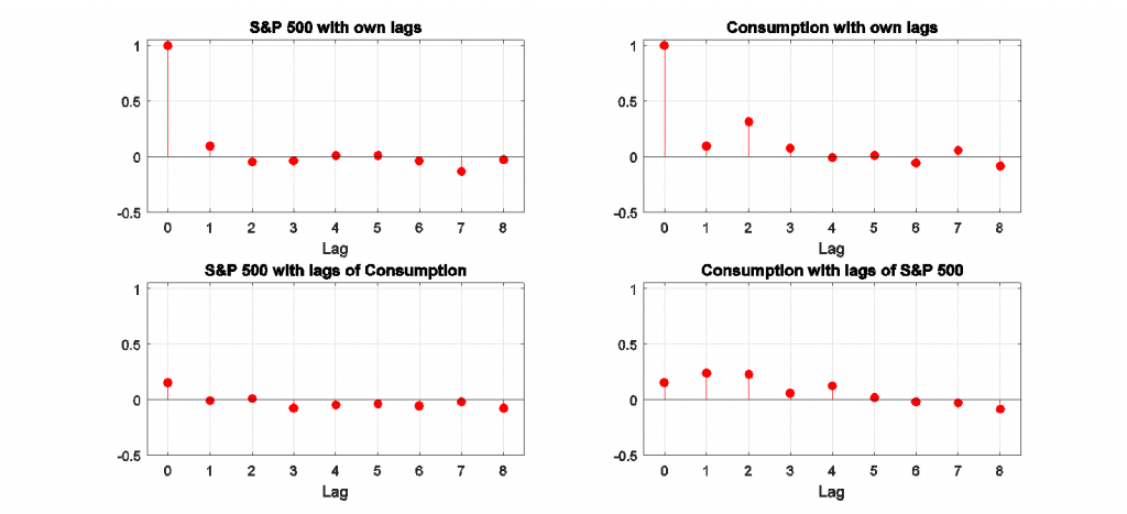
Autocorrelations and cross-correlations for first-difference of stock prices and real consumption spending. Source: Hamilton (2016).

By contrast, here’s what the correlations look like for HP-detrended stock prices and consumption. As I note in the paper:

The rich dynamics in these series are purely an artifact of the filter itself and tell us nothing about the underlying data-generating process. Filtering takes us from the very clean understanding of the true properties of these series that we can easily see in the first figure to the artificial set of relations that appear in the second. The values plotted in the second figure summarize the filter, not the data.

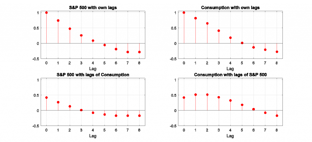
Autocorrelations and cross-correlations for HP-detrended stock prices and real consumption spending Source:Hamilton (2016).

There is one rather special case for which the HP filter is known to be optimal, which is if the second difference of the trend and the difference between the observed variable and its trend are both impossible to forecast. However, I show in my paper that if you took that specification seriously, you could estimate from the data the value for the smoothing parameter that would be consistent with the observed data. I found that when I did this for a dozen common economic variables, the implied value for the smoothing parameter is around one, which is three orders of magnitude smaller than the value of 1600 that everyone uses.

But the real contribution of my paper is to suggest that there’s a better way to do all this. I propose that we should define the trend as the component that we could predict two years in advance, and the cyclical component as the error associated with that two-year-ahead forecast. But don’t you need to know the nature of the trend in order to form this forecast? The surprising answer is no, you don’t.

The basic insight is that if 

 is stationary for some value of d, then you can write the value of the variable at date t + h as a linear function of the d most recent values of y as of date t plus something that is stationary. If you do a simple regression of yt+h on a constant on the d most recent values of y as of date t, the regression will end up estimating that linear function. The reason is that for those coefficients the residuals are stationary, while for any other coefficients the residuals would be nonstationary. Choosing coefficients to minimize the sum of squared residuals (which is what regression does) will try to find the coefficients that take out the trend, whatever it might be.

But what if we don’t know the true value of d? That’s again no problem. If we regress yt+hon a constant and the p most recent values of y as of date t for any p > d, , then d of the estimated coefficients will be used to uncover the trend and the other coefficients will help with forecasting the stationary component. If we use p = 4, we have the same flexibility of the HP filter (it can remove the trend even if we need 4 differences to do so), but without all the problems.

In the case of a random walk, we know analytically what this calculation would be. If the change is unpredictable, then the error you make predicting the variable h quarters ahead is just the sum of the changes over those h quarters. The easy way to calculate that sum is to just take the difference between yt+h and yt.

The figure below illustrates how this works for nonfarm payroll employment. The raw data are plotted in the top panel, and the cyclical or detrended component is in the bottom panel. I calculated the latter using both the residuals from a regression of yt+8 on a constant and yt, yt-1, yt-2, yt-3 (shown in black) and using just the sum of the changes between date t and t+8 (in red). The latter two series behave very similarly, as I have found to be the case for most of the economic variables I have looked at.

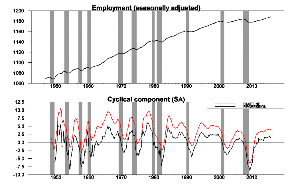
Upper panel: 100 times the log of end-of-quarter values for seasonally adjusted nonfarm payrolls. Bottom panel: residuals from a regression of yt+8 on a constant and yt, yt-1, yt-2, yt-3 (in black) and value of yt+8 – yt (in red). Shaded regions represent NBER recession dates. Source: Hamilton (2016).

One interesting observation is that the cyclical component of employment starts to decline significantly before the NBER business cycle peak for essentially every recession. Note that, unlike patterns one might see in HP-filtered data, this is summarizing a true feature of the data and is not an artifact of any forward-looking aspect of the filter.

Another benefit of this approach is that it will take out the seasonal component along with the trend. For example, the next figure shows the effects of applying the identical procedure to seasonally unadjusted employment data. The raw data (top panel) have a very striking seasonal component, whereas the estimated cyclical component (bottom panel) is practically identical to that derived from seasonally unadjusted data.

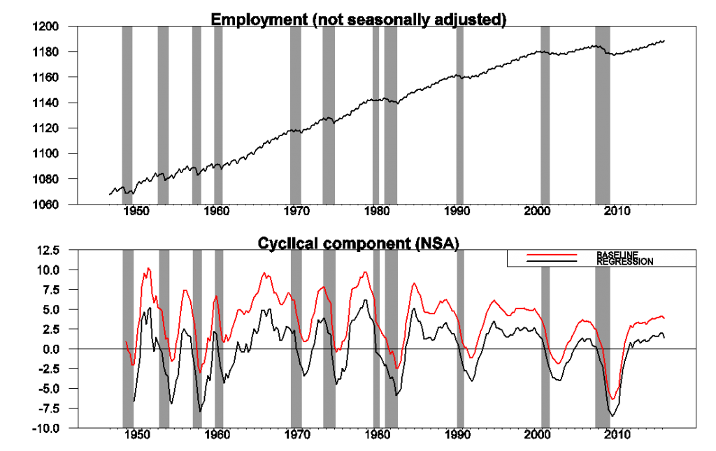
Source: Hamilton (2016).

The following graphs show the detrended behavior of the main components of U.S. real GDP. As I note in the paper,

Investment spending is more cyclically volatile than GDP, while consumption spending is less so. Imports fall significantly during recessions, reflecting lower spending by U.S. residents on imported goods, and exports substantially less so, reflecting the fact that international downturns are often decoupled from those in the U.S. Detrended government spending is dominated by war-related expenditures– the Korean War in the early 1950s, the Vietnam War in the 1970s, and the Reagan military build-up in the 1980s.

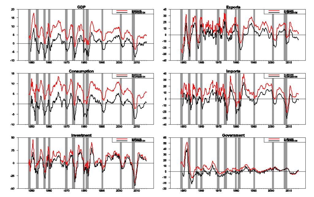
Source: Hamilton (2016).

Here’s a slight rephrasing of the paper’s conclusion:

The HP filter will extract a stationary component from a series whose fourth difference is stationary, but at a great cost. It introduces spurious dynamic relations that are purely an artifact of the filter and have no basis in the true data-generating process, and there exists no plausible data-generating process for which common popular practice would provide an optimal decomposition into trend and cycle. There is an alternative approach that can also isolate a stationary component from any series whose fourth difference is stationary but that preserves the underlying dynamic relations and consistently estimates well defined population characteristics for a broad class of possible data-generating processes.