Factors In Long-Term Unemployment

The BLS reported on Friday that the U.S. unemployment rate was down to 5% in October and November, its lowest level since 2008.

The dramatic surge in unemployment during the Great Recession and its stubborn persistence in coming back down were both dominated by a tremendous increase in the number of people who spent longer than six months looking for a job. If we only counted individuals searching for six months or less, the unemployment rate today would be 3.7%, near the lowest levels for that measure over the last half century.

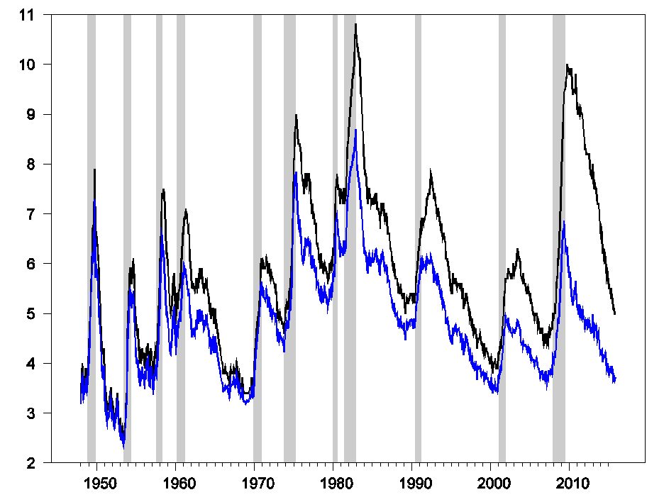
Figure 1. Seasonally adjusted number of people unemployed as a percent of the labor force (or the usual unemployment rate, in black) and number of people who were unemployed for 6 months or less as a percent of the labor force (blue). Latter calculated by multiplying unemployment rate by one minus the fraction unemployed for 27 weeks or longer.

One of the best predictors of whether an individual who is unemployed today will still be unemployed next month is how long that individual has already been looking for a job. For most of the last 50 years, if you considered an individual who has only been looking for work for one month, more likely than not you would find that individual was no longer unemployed the following month. But in every year of the sample, if you looked at an individual who had already been looking for work for longer than six months, there would be a better than an 80% chance that individual would still be unemployed the following month.

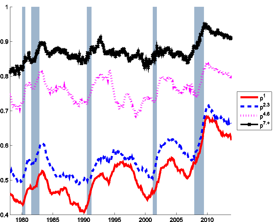
Figure 2. Probability that an unemployed individual will still be unemployed the following month for different durations of job search, Jan 1976 to Dec 2013. Red: individuals who have been unemployed for less than 1 month as of the indicated month; blue: unemployed for 2-3 months; fuchsia: 4-6 months; black: longer than 6 months. Calculated as described in foonote 1 in Ahn and Hamilton (2015).

One possibility is that the process of being unemployed for longer than a month actually changes an individual through some kind of scarring effect. For example, employers may start to discriminate against those who have been out of work for longer. Another possibility is that there are important differences across individuals that began in their very first month without a job, with some people having less favorable skills and opportunities. If you follow those individuals over time, the ones who are still looking after six months will be selectively drawn from those who had a much lower probability of finding a job from the very beginning.

You can see how this could happen with a simple example. Suppose that in a given group of 100 newly unemployed individuals, 20 of them are “type L”, who have an 85% chance of still being unemployed next month, while the other 80 are “type H”, who only have a 35% chance of remaining unemployed. After one month of searching, 17 of the type L (85% of the original 20) will still be looking for work, compared with 28 of type H (35% of the original 80). Of the people who are still searching after 2 months, 60% (15/25) will be type L, even though they were only 20% of the original 100. After 6 months, 9 of the original 100 may still be looking for work, and they are almost certain all to be type L.

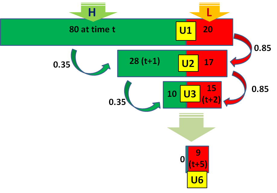
Figure 3.

We can get a quick idea of plausible numbers from the following calculation. Suppose that in an average month there are w_L newly unemployed type L individuals and that their average probability of still being unemployed next month is p_L (in the above example, p_L was assumed to be 0.85). Then the average number of type L individuals who have been looking for work for k months would be w_L x p_L^k-1. The average number of type H individuals who have been looking for work for k months would similarly be w_H x p_H^k-1. If there’s no way to determine an individual’s type from the information recorded in BLS data, then all we would observe would be the total number of people who have been looking for work for k months, which would be the sum of the above two numbers:

U(k) = w_L x p_L^k-1 + w_H x p_H^k-1.

Suppose we observe the average number of individuals looking for work at 4 different values of k, represented by the first 4 dots in Figure 4 below. We could then use these four observed values to calculate values for the 4 unknowns w_L, p_L, w_H, and p_H. For example, the average number of newly unemployed individuals, U(1) = 3.2 million, must equal the sum of w_L + w_H, as illustrated in the figure.

Figure 4. Horizontal axis shows duration of unemployment in months and vertical axis shows number of unemployed for that duration in thousands of individuals. Dots correspond to average observed numbers for selected durations over the period Jan 1976 to Dec 2013. Source: Ahn and Hamilton (2015).

The values for p_L and p_H that result from this curve-fitting are 0.85 and 0.36, essentially those used in the red-green diagram above. The imputed fraction of type L individuals among the newly unemployed is 21%. The calculation also gives a predicted value for the fifth dot in Figure 4, corresponding to the average number of longer-term unemployed individuals, that turns out to be very close to what we observe in the data.

Now suppose that we were to redo the exercise using only data since December 2007. The result is summarized in Figure 5. The average number of newly unemployed individuals, 3.3 million, is only slightly higher than the historical average. The unemployment-continuation probability for type L individuals is estimated to be 0.89, again only a little higher than that for the historical average. The feature of the data that gives rise to this conclusion is that the average numbers of longer-term unemployed individuals drops off only slightly slower than they did historically. But we’d be forced from this calculation to conclude that many more type L individuals have been losing their jobs since 2007 than had historically been the case. The exercise suggests that while there were 680,000 newly unemployed type L individuals on average each month over the entire sample, since 2007 the inflow has been over a million each month.

Figure 5. Dots correspond to average observed numbers for selected durations over the period Dec 2007 to Dec 2013. Source: Ahn and Hamilton (2015).

Why might the composition of the pool of newly unemployed have changred during the Great Recession? One reason could be that firms decide which individuals to lay off during a recession based on how they have been performing at the job. More importantly, the skills sought by all employers could change with changing business conditions. For example, an unemployed carpenter might behave like a type H individual during a housing boom, quickly finding another job. But during an economy-wide housing bust, it will be much more difficult for that same person to find a job. Under either explanation, type L individuals would make up a bigger share of the newly unemployed during a recession compared to normal times.

In a recent paper with Hie Joo Ahn, a former student of mine who is now an economist at the Federal Reserve Board, we studied a generalization of the above model in which the magnitudes w_Lt, p_Lt, w_Ht, and p_Ht could all be changing every month t. In addition we allowed the possibility that there could be a separate scarring or discrimination effect arising from a longer spell of unemployment itself. The resulting inferences for the unemployment-continuation probabilities p_Lt and p_Ht are plotted in Figure 6. These average 81% and 34%, respectively, consistent with the quick calculations above. The value of p_Lt shows a modest tendency to increase during recessions and remain higher after the Great Recession.

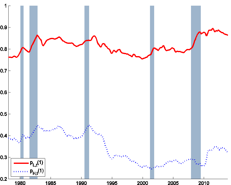
Figure 6. Probability that a newly unemployed individual of each type will still be unemployed the following month. Source: Ahn and Hamilton (2015).

Figure 7 shows our estimates of w_Lt and w_Ht, the new inflows into unemployment of each type. Type L individuals represent only 21% of the newly unemployed on average, again consistent with the above quick estimates. There is a big increase in this magnitude during each recession and particularly dramatically so during the Great Recession.

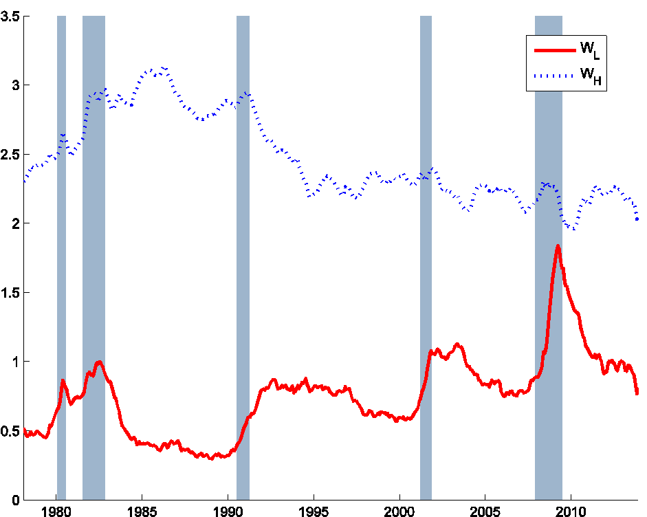
Figure 7. Number of newly unemployed individuals of each type. Source: Ahn and Hamilton (2015).

Could these same patterns instead be explained from the scarring or discrimination effect of being unemployed mentioned above? A recent survey by Krueger, Cramer, and Cho (2014) concluded that it might, pointing for example to experiments by Kroft, Lange, and Notowidigdo (2013) who found that potential employers were less likely to call back on fictitious resumes with longer reported unemployment. But an audit study by Farber, Silverman, and von Wachter (2015) failed to confirm those findings, while Jarosch and Pilossoph (2015) built a model in which effects of the size found by Kroft and coauthors could be almost entirely accounted for by the information that unemployment duration gives about true worker characteristics. Alvarez, Borovickova, and Shimer (2015) found from a dataset following individual Austrian workers over long periods that unobserved characteristics specific to individuals rather than effects of unemployment itself were the key determinant of unemployment durations. In my paper with Hie Joo Ahn we were able to use variation over time in aggregate counts of unemployment by duration to allow for both a quite general scarring effect as well as cyclical variation in unobserved worker characteristics and found that the latter was far more important quantitatively.

Another reason that Krueger and others are skeptical of this possibility is that we do not see significant changes in observable characteristics of the long-term unemployed during recessions. But Ahn (2015) demonstrated that within any group of individuals with the same coarse observable characteristics we find a similar pattern to that in Figures 4 and 7 above. The conclusion is that there are different unobserved types of individuals within every group of people sharing a giving observed characteristic.

Even so, there are some important regularities we can document based on observable characteristics. Type L individuals are more common among those who involuntarily lose permanent jobs, and cyclical variation in permanent job losses seems to be a key factor responsible for cyclical variation in w_Lt. Changes in the composition of the newly unemployed based on whether they were permanently separated and whether they file a claim for unemployment insurance turn out to be strong predictors of subsequent levels of aggregate unemployment over and above the aggregate new inflows into unemployment.

Though it might have seemed like a natural hypothesis, ours is the first paper to document the cyclical importance of this unobserved heterogeneity across individuals. We conclude that this phenomena is absolutely crucial for understanding cyclical fluctuations in unemployment.