<< Read Part I: To Log Or Not To Log

Following up on this post, estimating the consumption function.

Consider the canonical consumption-income relationship discussed in macro textbooks. For pedagogical reasons, the relationship is often stated as:

(1)   C = c0 + c1 Yd

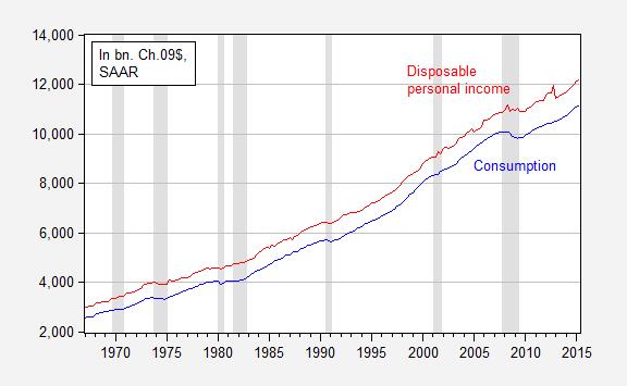
Where C is real consumption and Yd is real disposable income. Figure 1 depicts the relationship over the 1967-2015Q2 period.

Figure 1: Consumption (blue) and disposable personal income (red), in billions of Ch.2009$, SAAR. NBER defined recession dates shaded gray. Source: BEA, 2015Q2 advance release, and NBER.

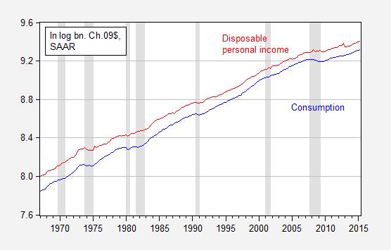
Now consider the corresponding figure, in logs.

Figure 2: Log consumption (blue) and log disposable personal income (red), in billions of Ch.2009$, SAAR. NBER defined recession dates shaded gray. Source: BEA, 2015Q2 advance release, and NBER.

It does seem hard to choose one over the other merely by looking. Reader Mike V writes:

I just think you lose a lot of people by using logs for every. graph.

Which one is the better way to characterize the relationship? At first glance, estimating each by way of OLS does not allow much to distinguish between the two. In levels:

(2)   C = -336.7 + 0.945Yd

R2 = 0.999, SER = 93.26, Nobs = 194, DW = 0.56. Bold Face indicates significance at 5% msl using HAC standard errors.

In logs:

(3)   c = -0.651 + 1.061yd

R2 = 0.999, SER = 0.014, Nobs = 194, DW = 0.48. Bold Face indicates significance at 5% msl using HAC standard errors.

Clearly, neither specification is adequate, but is one to be preferred to another? Theory does not provide guidance, as the linear consumption function is typically used for convenience.

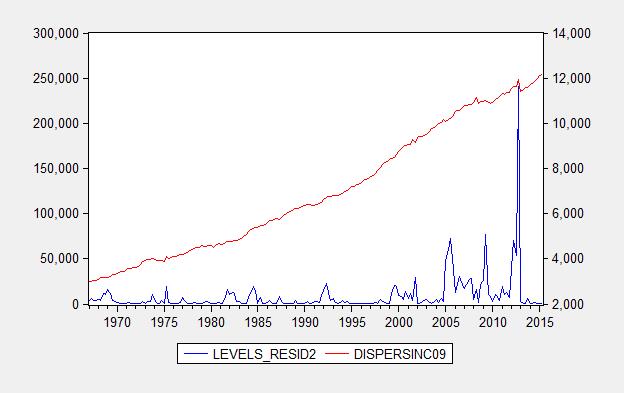
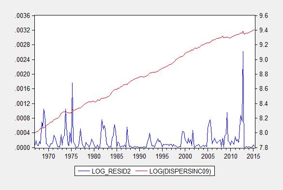
One factor one can use to inform a choice is heteroscedasticity, the characteristic wherein the variance of the errors is not constant. One does not observe the true residuals, but one can examine the squared estimated residuals, and see if there is a systematic pattern between the squared residuals and the right hand side variable. Figure 3 presents the squared residuals from the levels specification, and Figure 4 presents squared residuals from the log specification.

Figure 3: Squared residuals from levels regression (2).

Figure 4: Squared residuals from log levels regression (3).

While in both cases the residuals exhibit a (positive) correlation with the right hand side variable, it is much more pronounced in the levels regression. In other words, the real dollar errors increase systematically with real dollar disposable income, while (log) percent errors increase less strongly with percent increases in real disposable income. This provides one reason to prefer a log specification. By the way, a Jarque-Bera test rejects normality for both residuals, but much more soundly for the levels specification.

Now, the residuals exhibit substantial serial correlation (rule of thumb: possible spurious correlation of integrated series if the R2 > DW). This suggests estimating a cointegrating relationship (see this post) or – if one wants the short run dynamics – an error correction model. The analogs to equations (2) and (3) (after augmenting with household net worth to account for life-cycle effects) are:

(4)   ΔCt = 1.900 + 0.027Ct-1 – 0.018Yd,t-1 – 0.0008Wt-1 + lagged first difference terms

R2 = 0.25, SER = 33.55, Nobs = 192, DW = 2.21. Bold Face indicates significance at 5% msl.

In logs:

(5)   Δct = 0.014 – 0.017ct-1 + 0.011 –yd,t-1 + 0.004wt-1 + lagged first difference terms

R2 = 0.21, SER = 0.006, Nobs = 192, DW = 2.18. Bold Face indicates significance at 5% msl.

In this case, there is no clear advantage to one specification or the other. The levels specification indicates explosive behavior (as the coefficient on the lagged level of the dependent variable is positive; but it’s not statistically significant). Only the lagged differenced variables are statistically significant. In the log specification, the implied behavior is not explosive, given the coefficient on the lagged log level of the dependent variable; actually given the non-significance of the coefficient, there does not appear to be evidence of cointegration (actually, all that we know is that consumption does not seem to revert to re-establish the long run relationship between consumption, income and wealth – it might be that the other two variables do the adjustment, and in fact a Johansen test suggests this is the case).

For a more detailed analysis, disaggregating consumption data, see this post. In that case, logs in conjunction with disaggregation seems to do the trick.

>> Read Part III: To Log Or Not To Log, Part III