The Bureau of Economic Analysis announced today that seasonally adjusted U.S. real GDP grew at a 2% annual rate in the third quarter, slightly below the average growth rate of 2.25% that we saw during the previous economic expansion.

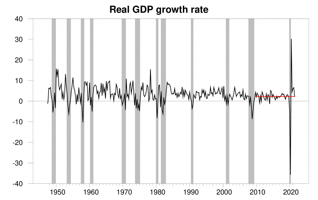
Real GDP growth at an annual rate, 1947:Q2-2021:Q3, with the 2009:3-2019:4 average (2.25%) in red. Calculated as 400 times the difference in the natural log of GDP from the previous quarter.

The new data put the Econbrowser recession indicator index at 0.3%, historically a very low value and signaling an unambiguous continuation of the economic expansion. The number posted today (0.3%) is an assessment of the situation of the economy in the previous quarter (namely 2021:Q2). We use the one-quarter lag to allow for data revisions and to gain better precision. This index provides the basis for an automatic procedure that we have been implementing for 15 years for assigning dates for the first and last quarters of economic recessions. As we announced on January 28, the COVID recession ended in the second quarter of 2020. The NBER Business Cycle Dating Committee subsequently made the same announcement on July 19.

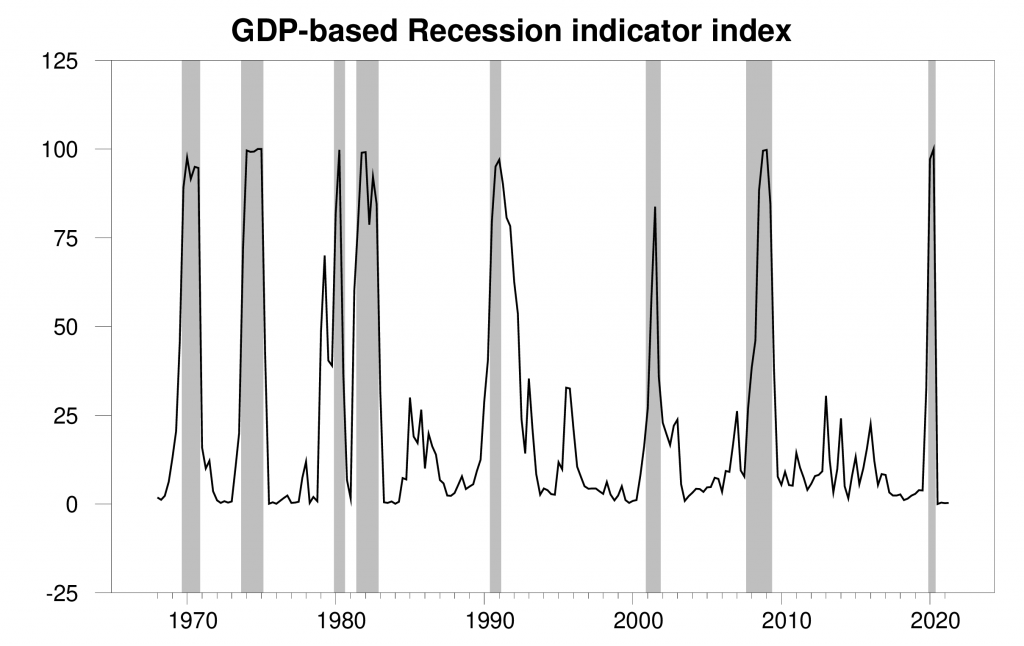
GDP-based recession indicator index. The plotted value for each date is based solely on the GDP numbers that were publicly available as of one quarter after the indicated date, with 2021:Q2 the last date shown on the graph. Shaded regions represent the NBER’s dates for recessions, which dates were not used in any way in constructing the index.

By Q2, the level of GDP had recovered to the value reached in 2019:Q4 before the COVID recession began. But if we hoped to return to the trend line associated with the previous expansion (shown in red in the graph below), we’d need to see growth for Q3 of over 4%, not 2%, and we’d have to maintain that pace for a full year.

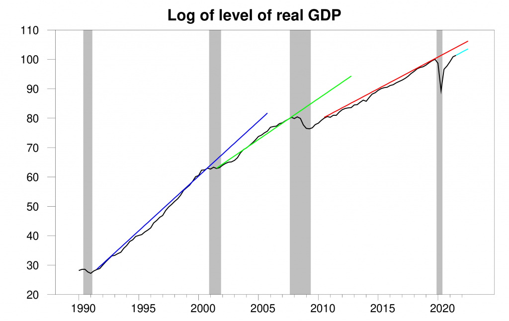
100 times the natural logarithm of the level of real GDP, 1990:Q1 to 2021:Q3, normalized at 2019:Q4 = 100. A movement on the vertical axis of 1 unit corresponds to a 1% change in the level of real GDP. Blue line extrapolates the trend from the 1991-2000 expansion, green from the 2001-2007 expansion, and red from the 2010-2019 expansion.

But the expectation that we’ll recover to the previous trend once a recession is over doesn’t have much support in the data. Economic recessions seem to have permanent effects on the level of GDP. There is often above-average growth in the first few quarters of expansion (the recovery phase in a “V” shape). But once the level of GDP is back to its pre-recession value, trend growth becomes the norm. We also see in the above graph that the average growth rates during expansions (which determine the slopes of the lines) seem to be falling over time. Big factors in those falling average growth rates are slower growth of the labor force and productivity.

In terms of the individual components of GDP, a key reason that the economy grew at only a 2% rate in Q3 is slower growth in consumption spending. Purchases of automobiles were a big factor in this. An important cause is difficulties car manufacturers are having in acquiring the computer chips required to put together the modern car.

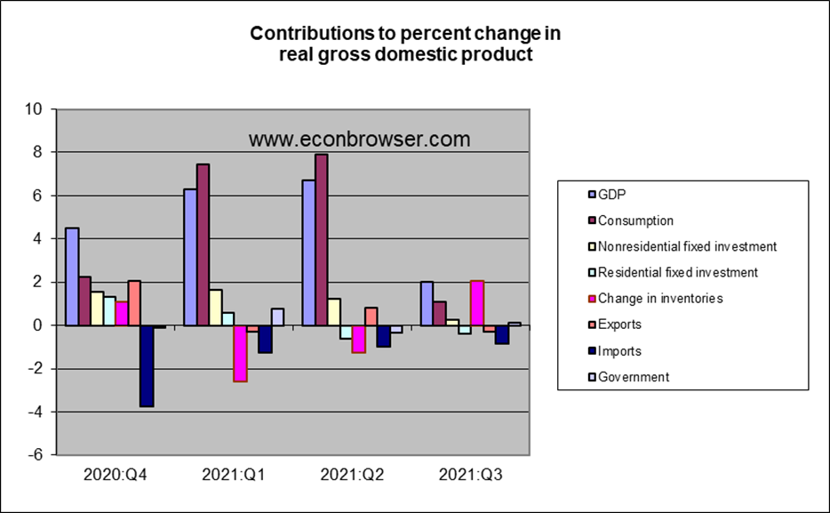
Another disappointment was new home construction, which made a negative contribution to the Q3 growth rate. We’ve seen plenty of stimulus for more residential fixed investment with low interest rates and dramatically rising house prices. Some analysts are also blaming sluggish new home construction in part on supply-side problems.

Inventory changes were an even bigger factor in the GDP numbers. If inventory investment had not made a positive contribution, GDP in Q3 would actually have declined relative to Q2. To understand what this means, it’s important to remember the way that inventories enter the GDP accounts. The change in inventories during a quarter is referred to as inventory investment. If inventories end up higher than they started out, inventory investment is positive, and if inventories are lower than they started out, inventory investment is negative. Inventory investment was sharply negative in Q2 of this year (namely -$174B at a quarterly rate). Inventory investment was still negative in Q3 (namely, -$68B), but not as negative as in Q2. Thus inventory investment was $106B higher in Q3 than it had been in Q2 (-68 – (-174) = +106). This alone accounts for essentially all of the increase in GDP between Q2 and Q3.

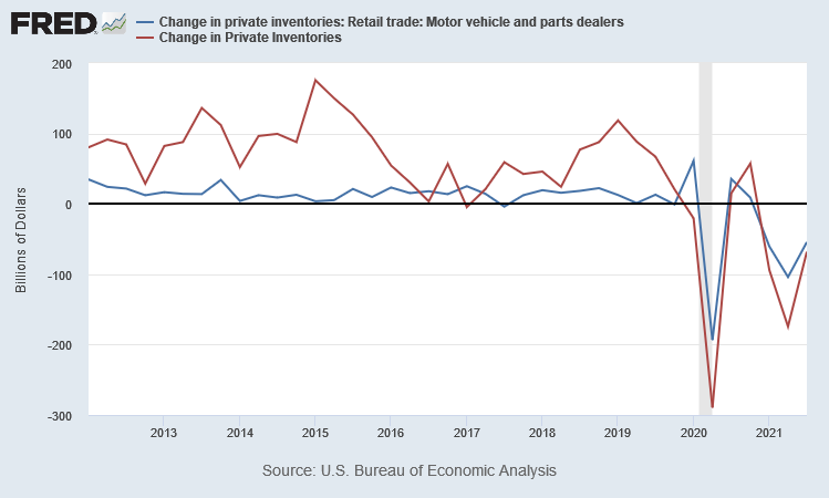
Nominal inventory investment, quoted at a quarterly rate, 2012:Q1-2021:Q3. Red line: Change in dollar value of all private inventories. Blue line: change in dollar value of inventories of dealers of motor vehicles and parts.

The graph above also shows where these inventory movements come from: cars are the main story. The manufacturers weren’t delivering enough new cars to dealers, which is why inventories ended the quarter lower than they started. This is another important way that the car-makers’ supply-chain issues are having big effects on U.S. GDP.

As these supply-side constraints ease, I would expect to see a surge in both consumer purchases and dealer restocking. Both changes should give a big boost to GDP. So it might be that 4% rather than 2% is the kind of growth we should be expecting once supply problems ease.

But fiscal and monetary stimulus are not the policies we should be looking for to get us to that faster economic growth.