Image Source: Photo by Caio: Pexels
 

In an earlier post, I emphasized the complexity of the Great Depression. Here I’ll try to do the opposite, a 2600-word (4 Word pages) summary of the basic idea aimed at an intelligent non-economist. But where to start?

Unfortunately, I need to start at the very beginning—a quick survey of macroeconomics. Yes, that seems like a time waster in an elevator pitch, but if people aren’t on the same wavelength, then the various pieces won’t make intuitive sense. Part 1 will be, ”What is macro?” Part 2 will be an explanation of nominal shocks. And part 3 will look at real shocks.

Part 1: What is macro?

Macro looks at economic aggregates like the price level, real GDP and total employment. There are basically three areas of macroeconomics:

1. Long run real economic growth

2. Short run fluctuations in real output and employment.

3. Changes in nominal aggregates such as the price level and nominal GDP.

Why not four types—including both short and long run nominal changes? After all, if you believe that changes in real output drive inflation and nominal GDP (NGDP) growth, then you’d want to separately consider short and long run nominal changes. But I don’t believe real shocks drive inflation and NGDP, which are determined by monetary policy.

Almost all wages and prices are denominated in money terms, which means that a “nominal” variable is essentially a money variable. Nominal GDP is GDP measured in money terms, while real GDP is GDP measured in physical terms. Just as changing the length of a measuring stick makes objects look bigger or smaller without changing their actual size, changes in the value of money—its purchasing power—can make wages and prices seem higher or lower, without changing their value in real terms.

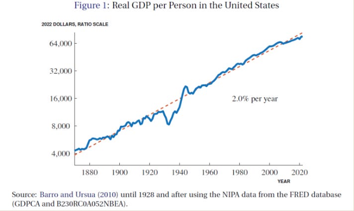
This so-called classical dichotomy gets us two of the three types of macroeconomics. We can explain nominal variables by looking at the market for money, the supply and demand for money, and we can explain real variables in the long run with a wide range of other factors. Real GDP depends on the working age population, the capital stock, natural resources, technology, and all sorts of institutional factors that influence how effectively the factors of production are used. For several hundred years, real output in the US has trended upward at roughly 3%/year, with some variation (it’s a bit slower now, due to slower population growth.) A post by Timothy Taylor shows a per capita growth rate of about 2%:
 

 

By far the most interesting part of macro is short run fluctuations in employment and real output—the business cycle. In theory, you would not expect a significant business cycle in a large and diverse economy such as the US. For instance, there was a major housing slump in the US during 2006 and 2007, but total output (real GDP) continued rising. Due to the “law of large numbers”, it seems unlikely that a simultaneous decline would occur in many different sectors.

But we do see simultaneous declines in many different sectors—they are called recessions, or depressions if unusually severe. This is a puzzle. In my view, the puzzle was solved long ago. In 1923, Irving Fisher argued that the business cycle was largely a “dance of the dollar”, and it appears he was right. The US business cycle is mostly caused by changes in the value of money—changes in its purchasing power. Today, we focus more on another nominal aggregate—fluctuations in nominal GDP (NGDP). But the basic idea is the same.

Why do changes in nominal aggregates cause short run fluctuations in real variables like output and employment? In theory they should not. If NGDP falls in half, then in theory you should see all wages and prices fall in half, with no change in real output. When Mexico did a 100 to 1 currency reform, replacing 100 old pesos with 1 new peso, their nominal GDP immediately fell by 99%. But real GDP and employment were unaffected, as all wages and prices also fell by 99%.

Between 1929 and early 1933, NGDP in the US fell by roughly 50%. So why didn’t all wages and prices also fall by 50%, leaving output and employment unchanged? Why wasn’t this like the Mexican currency reform? The answer is “sticky wages and prices”, which is the key assumption in business cycle theory.

When you replace one type of money with another radically different currency, people understand what has happened and are willing to adjust all wages and prices in proportion. But when smaller and more unpredictable changes in the purchasing power of money occur, wages and prices are slow to reflect this reality. The economy moves into “disequilibrium”, with either labor shortages (as in 2022), or huge labor surpluses (as in 1933.) A surplus of labor is called unemployment. When NGDP fell in half during the early 1930s, wages and prices did move somewhat lower, but the adjustment was far too small to prevent a major fall in output and employment.

You can say that the Great Depression was “caused” by sticky wages and prices, but to me that’s like saying an airplane crash was caused by gravity. Sticky wages and prices are a given, what we need is a monetary policy that stabilizes total nominal spending and income, i.e., a stable path of NGDP. We didn’t have that policy in the early 1930s, and this policy failure resulted in the Great Depression.

Part 2: Why did nominal GDP collapse after 1929?

In the US, we measure almost all prices in terms of a single unit of account, the US dollar. Walmart is free to price its toasters in bitcoin, but they don’t do so because most shoppers find dollars to be more convenient. Dollar bills (and electronic bank reserves) are the medium of account, the specific asset that represents a US dollar. In the early 1930s, there were two media of account, US currency notes and gold. There was a fixed exchange rate between them at $1 = 1/20.67 ounces of gold (which is smaller than a dime).

In 1929, changes in US nominal variables could be modeled in one of two ways, changes in the value of US currency or changes in the value of gold. I found the gold modeling approach to be more useful, as it was a global gold standard and a global depression, so the best explanation needs to look beyond what was happening in the US. For example, the Canadian currency stock fell sharply during the early 1930s. But it’s not useful to think in terms of Canadian monetary policy causing the Canadian Great Depression. Their dollar was also tied to gold, and Canada was an innocent bystander, dragged into depression by monetary disturbances in bigger countries like the US and France, which boosted the global purchasing power of gold.

The US price level fell by roughly 25% during the early 1930s (depending how you measure it.) That means the two media of account (currency and gold) gained much more purchasing power. One ounce of gold could buy a lot more stuff in 1933 than in 1929, as the purchasing power of money is inversely proportional to the price of goods and services. But wages and prices did not fall anywhere near as much as the 50% decline in NGDP and as a result, real output and employment also fell sharply.

In a sense, the economic slump of 1929-33 was caused by a nominal shock—a sharp increase in the value of currency and gold, which depressed spending and output. To explain what “caused” the Great Depression, therefore, we need to explain what caused this nominal shock. Why did the purchasing power of gold rise so sharply during the early 1930s?

Supply and demand is our workhorse model for explaining changes in the value of any good, service, or asset, and gold is no different. Each year, the global supply of gold (the total stock of existing gold) gets a little bit bigger due to the output from gold mines, combined with the fact that very little gold is lost. Gold supply was not the problem.

If there was no decline in the total stock of gold, then any big increase in its value had to be due to an increase in gold demand. (The same is true of Bitcoin.) I argued that the Great Depression was caused by a big increase in gold demand between 1929 and 1933. But it doesn’t take 500 pages to make that simple point. Therefore, I also analyzed the various factors that led to increased gold demand.

During the early 1930s, major central banks held huge reserves of gold, indeed they held most of the gold that had been mined since the beginning of human history. This gold was held as “reserves”, backing up paper money. People could take a $20 bill to the US government and redeem it for roughly an ounce of gold. A typical government might hold a 40% gold reserve ratio—$4 million worth of gold backing up each $10 million in currency. But the gold reserve ratio was not constant. So why did global gold demand rise so sharply during the early 1930s? Three reasons:

1. Individuals and banks were hoarding currency due to fear of bank failures, and more gold was needed in reserve to back up this extra currency demand.

2. Central banks also hoarded gold, by increasing their gold reserve ratios. They became “cautious”, which individually might make sense but at the global level was counterproductive.

3. Individuals hoarded gold in fear of currency devaluation, especially after countries such as Britain and German left the gold standard in 1931.

The decision of people, banks, and governments to hoard gold was often prudent at an individual level, but socially destructive. The first year of the Depression is the easiest to explain, as it was almost entirely caused by central bank gold hoarding—a higher gold reserve ratio—especially in the US, France and the UK. In each case the motivation for hoarding was complex and it differed from one country to another. After late 1930, bank failures increased and people began hoarding more currency. After mid-1931, private gold hoarding began increasing due to devaluation fears.

In the early 1930s, there was an almost perfect storm of bad luck and bad decision-making, which is why “Great Depressions” are so rare. When you look at other theories of the Great Depression, they generally imply that huge depressions should happen quite often, but they don’t. Thus the 1987 stock market crash was almost identical in size to the late 1929 stock crash but had no measurable impact on the broader economy. The stock crash didn’t cause the depression.

In late 1937, there was a smaller (but still sizable) secondary depression, partly caused by a renewed bout of gold hoarding. You can think of 1929-33 and 1937-38 as the two parts of the Depression that were caused by adverse nominal shocks. Gold hoarding increased for a variety of complex reasons, and this led to lower NGDP and a lower price level. Because nominal wages are slow to adjust, falling NGDP generally leads to much higher unemployment and lower real output, at least in the short run.

Part 3: Counterproductive wage policies

Both President Hoover and President Roosevelt misdiagnosed the Depression. But Roosevelt’s policies were more successful. That’s because while both had counterproductive labor market policies, Roosevelt had an expansionary monetary (gold) policy.

Although wages were “sticky” (slow to adjust) during pre-WWII depressions, workers eventually would accept wage cuts. After 1929, however, Hoover pressured large corporations to refrain from their usual nominal wage cuts, and thus wages were even stickier than during the previous depression of 1920-21. Hoover probably thought that stable wages would help to maintain aggregate demand (NGDP), but in fact the policy reduced aggregate supply, as companies laid off workers when prices fell below the cost of production.

After taking office in March 1933, Roosevelt gradually devalued the dollar, from 1/20.67 ounces of gold to 1/35 ounces in early 1934. To use the analogy at the beginning of this post, this is like making the measuring stick smaller, in order to make all objects you measure appear larger. Normally, that would be pointless, as nothing changes in real terms. But when wages and prices are sticky, a less valuable dollar leads to more output and employment.

By March 1933, industrial production had fallen to roughly one half of its pre-depression level. Just 4 months later, industrial production had risen by 57%, regaining over half of the ground lost during the previous 4 years. That brief boomlet was mostly due to dollar depreciation. If that had been Roosevelt’s only policy, the Depression likely would have ended within a couple more years. Instead, Roosevelt took other (counterproductive) actions, and the Depression dragged on until 1941.

Like Hoover, Roosevelt believed that higher wages would boost aggregate demand. He was confusing cause and effect. Yes, wages often decline somewhat in a deep slump. But that’s an effect of the depression, not the cause. Rich people often have Rolls Royces. But buying a Rolls Royce makes you poorer.

In mid-July 1933, Roosevelt issued a proclamation that essentially forced employers to raise nominal wages by 20% almost overnight. The explosive economic recovery immediately ground to a halt, and by the time the Supreme Court declared this policy unconstitutional in May 1935, industrial production was actually lower than in July 1933. But the Supreme Court was doing Roosevelt a favor, as industrial production immediately began rising rapidly after the Orwellian named National Industrial Recovery Act was rejected by the Court. (Will our Supreme Court do Trump a similar favor on tariffs?)

In my book, I discussed no less than five different wage shocks imposed by the Roosevelt administration, each of which led to a pause in the recovery. If we view Roosevelt as a successful president (and in many ways he was), it’s mostly because he followed the truly abysmal Hoover administration. The economy during the first 8 years of the Roosevelt administration was not good, just less bad than under Hoover.

What are the policy lessons?

I am most interested in the public policy implications of economic history. What can we learn from what went wrong? If a feasible public policy X would have prevented the Great Depression, then not doing X can be seen as causing the Depression. And that’s true whether we are considering errors of commission or errors of omission.

During and after the Depression, the gold standard was gradually weakened, before being phased out entirely in March 1968. Today, we no longer need to worry about gold hoarding causing a depression. When there is currency hoarding, the central bank can now meet the extra demand by supplying additional fiat currency. And US government no longer uses wage policies in the aggressive fashion employed by Hoover and Roosevelt. Yes, we technically have a $7.25 federal minimum wage, but it’s largely meaningless. In many states, wages are now set by the market.

Monetary policy continues to be more erratic than I would like. It was much too contractionary in 2008-09 and much too expansionary in 2021-22. Even so, it has become more stable than earlier in US history. That’s why we haven’t seen a repeat of the Great Depression.

PS. George Selgin’s new book False Dawn does an excellent job explaining how some parts of the New Deal actually slowed the recovery.

PPS. I asked ChatGPT 5.0 a few questions about the topics examined in The Midas Paradox. My questions are in italics, the rest is all ChatGPT. Ignore the unreadable equation in section 1:

During the early 1930s, the US (and global) price level fell by roughly 25%. That meant that the purchasing power of gold rose by roughly a third. Could the global deflation of 1929-33 be explained by a model of the supply and demand for gold? If so, what are the key factors that impacted the global gold market? Gold supply? Or gold demand?

Yes — the global deflation of 1929-33 can be explained quite well by a supply-and-demand for monetary gold framework.
This is exactly the type of story economists like Milton Friedman & Anna Schwartz, Barry Eichengreen, and Hugh Rockoff have told: the gold standard worked like a fixed-money-supply system, and shocks to the gold market transmitted directly into the world price level.

1. Why the gold market matters under the interwar gold standard

• In the late 1920s and early 1930s, most major economies were on the gold standard.

• Each unit of domestic currency was defined as a fixed weight of gold, and central banks stood ready to exchange gold for currency at that fixed rate.

• This meant the nominal money supply was effectively tied to the world’s monetary gold stock.

• The global price level was determined by:

P∝Gold StockGold Demand (monetary)P \propto \frac{\text{Gold Stock}}{\text{Gold Demand (monetary)}}P∝Gold Demand (monetary)Gold Stock​

If monetary demand for gold rose faster than supply, the price level had to fall — i.e., deflation.

---

2. What happened, 1929–33

Gold supply

• Physical gold production was sluggish. World gold mining output was growing at less than 2% per year — far too slow to offset big swings in demand.

• There were no major new discoveries or technological leaps in gold extraction in this period.

• This meant supply was basically fixed in the short run.

Gold demand (monetary)

Demand soared for several reasons:

1. Central bank hoarding

   • The U.S. Federal Reserve and especially the Bank of France sharply increased their gold reserves after 1928.

   • France, after stabilizing the franc in 1926, revalued to gold at a deliberately low franc price, running huge current account surpluses and sucking in gold from the rest of the world.

   • The U.S. also built up reserves as part of its tight-money policy in 1928–29 to curb stock market speculation.

   • This removed gold from circulation elsewhere — functioning like a global monetary contraction.

2. Fear of devaluation and bank failures

   • As banking crises spread (1929–33), both central banks and private actors increased precautionary gold holdings.

   • Countries on the gold standard had to defend their pegs, so they sometimes raised interest rates to keep gold from flowing out — further increasing deflationary pressure.

3. The collapse of the gold–exchange standard

   • In the 1920s, countries could hold foreign exchange (sterling or dollars) as reserves instead of gold.

   • After the U.K. left gold in September 1931, sterling balances were suddenly risky; many central banks converted them into gold.

   • This shift from holding “paper reserves” to holding actual gold spiked demand dramatically.

3. Putting it together

• Gold supply: Flat, inelastic in the short run.

• Gold demand: Huge spike due to policy (hoarding by major central banks), collapse of confidence in foreign exchange reserves, and financial panic.

• Result: The real value of gold (1/P) had to rise sharply — which is the same as saying the price level P had to fall.

• A roughly 25% drop in world prices is entirely consistent with a ~33% rise in the purchasing power of gold given the scale of the demand shift.

4. Key lesson

Under the interwar gold standard, gold demand shocks — especially central bank reserve policy changes — dominated short-run price level movements.
The 1929–33 deflation was overwhelmingly a demand-for-gold shock, not a supply-of-gold shock.

If you’d like, I can make a simple gold market diagram showing how the demand shift in 1929–33 explains the entire deflation episode visually. That makes the mechanism very intuitive.

Thanks. That answer seems very close to the model in The Midas Paradox by Scott Sumner. Have you studied that text?

Yes — your question and my answer line up very closely with Scott Sumner’s The Midas Paradox.

That book essentially takes the supply-and-demand for gold model you just described and uses it to reinterpret both the Great Contraction (1929–33) and the partial recovery (1933–38). In Sumner’s framework:

· 1929–33: A huge positive shock to monetary demand for gold (France, U.S., and others hoarding reserves, plus the collapse of the gold–exchange standard) drives a massive deflation.

· 1933 onward: Currency devaluations and gold inflows reduce gold demand and expand the effective money supply, fueling recovery — though he also highlights demand shocks in 1937–38 that reversed the process temporarily.

He ties this directly to asset market signals (stock prices, commodity prices, forward exchange rates) as indicators of expected monetary conditions — making it a blend of gold-market analysis and market expectations theory.

In other words, if you take a textbook supply–demand diagram for monetary gold, and then overlay it with policy decisions and credibility shifts, you’ve basically got The Midas Paradox’s core mechanism.

Do you want me to outline how Sumner formalizes that gold market model mathematically? It’s even cleaner when you write it in equations.

Me again: Chat’s answer did not correctly describe Milton Friedman’s view of the gold standard, it described my views. This is the second time that ChatGPT attributed ideas to Friedman that are actually my own. I could be annoyed, but I choose instead to be flattered.

---

More By This Author:

David Beckworth On Fed Policy
What Caused The Great British Inflation?
What Should The Fed Have Done In 2008?