Reader Steven Kopits writes “potential GDP model is also a binding constraint model”, so GDP “…is subject to some sort of natural speed limit which cannot be exceeded”. This assertion is so amazingly absolutist in nature, and represents such a misunderstanding of how macroeconomists typically think of potential, that I am moved to observe that if this were so, output would never exceed potential GDP in our frameworks. Now, let’s consider the relevant depiction implied by the CBO estimates (using a production function approach [1]).

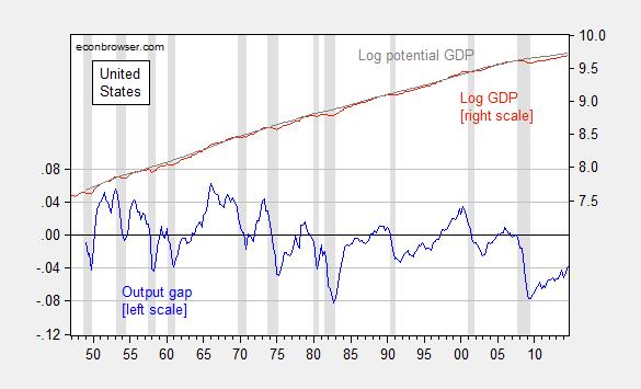
Figure 1: Log output gap (blue, left scale) and log GDP (red, right scale) and potential GDP (gray scale), all in bn. Ch.2009$, SAAR. NBER defined recession dates shaded gray. Source: BEA, 2014Q3 final release, CBO Budget and Economic Outlook (February 2014), NBER, and author’s calculations.

Note that output exceeds potential on numerous occasions according to CBO estimates, and hit 3.5% (log terms) as recently as in 2000. That’s because in this framework (the neoclassical synthesis, as forwarded in for instance Samuelson’s textbook, or e.g., here), factors of production can be utilized at greater than “normal” rates.

Now there are interpetations of potential GDP that fit Kopits’ description; from this post:

In Summers and Delong (1988), the authors provide an interpretation of potential as a level of output that can’t be exceeded (to me this is reminiscent of the Friedman “plucking model” (re-iterated in a 1993 publication, see also [1], [2])). Figure 5 depicts per capita potential under this interpretation.

 

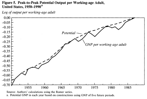
Figure 5 from Summers and Delong (1988).

The formula used is given by recursive application of their equation 17:

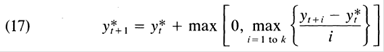
Where y* is potential GDP, and k=3 to 5. It’s of interest to consider what an updated version of the De Long-Summers procedure implies for the output gap. I apply the procedure to log GDP instead of per working age worker, and set k=3.

 

Figure 1: Log GDP (dark blue), CBO February 2013 projection (light blue), CBO potential, estimated by using 2011 ratio of 2009$ GDP to 2005$ GDP (gray), pseudo-DeLong-Summers (k=5) using actual data (dark red), and projection using CBO projections (pink). Source: BEA, CBO Budget and Economic Outlook (February 2013), and author’s calculations. [DeLong-Summers series calculation corrected 4:10pm]

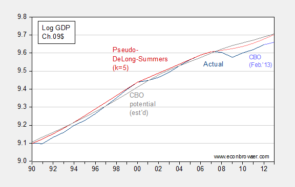
As of 2012, the output gap using the DeLong-Summers (1988) procedure is quite similar to the implied CBO gap — 3.1% vs. 4.3% (log terms). There are a couple of caveats.

First, the CBO has not released an estimate of potential that is consistent with the newly back-revised BEA GDP series. Hence, I have resorted to the expedient of adjusting the CBO potential GDP series by the ratio of actual GDP in 2011, expressed in 2009$ and 2005$ from the respective series.

Second, since the calculation of the DeLong-Summers procedure requires values of future growth, one can only calculate the 2012 value using estimates of 2013, 2014 and 2015 growth. In the figure above, I use the CBO’s February 2013 projections. The upward movement in the potential GDP in 2013 (and later, not shown) is due to the projected surge in GDP growth in 2015 and 2016 (in excess of 4%). If one were to forecast tepid growth in those years, the trajectory of the pink line would be depressed with a commensurately smaller output gap, in absolute value. (Setting k=4 or k=3 would also yield a different set of estimates.)

So, the implied degree of policy activism one should pursue in 2013 could differ substantially depending on views of the evolution of potential. Note that in Delong and Summers (2012), potential is endogenous, depending on the level of current economic activity (hysteresis effects, etc.), providing an additional reason for pursuing activist macroeconomic (specifically, fiscal) policies.

In the context of the DeLong-Summers framework, potential does constitute kind of a speed limit (although not completely since higher investment can increase the capital stock and hence elevate the trajectory of potential). But this speed limit interpretation does not apply for case for the conventional interpretation of potential GDP I use. Still plenty of wide, open road, and no speed limit in sight in this view.

I wish people would read an intermediate (heck, maybe an intro) macro textbook before saying what’s in the textbook…

For more discussion of how macroeconomists typically interpret potential, see this post, and Weidner, Williams/SF Fed. Notice that if one uses Mankiw’s approach of inverting the Phillips curve, the output gap is about -5.75% (log terms), even taking into account the upwardly revised GDP growth for 2014 Q3 in the final release.