

(This is intended as a primer on the use of systemic liquidity as tool in predicting the behavior of risk asset prices. It was first published in June 15, 2018).
Summary
The grand-daddy of systemic liquidity is, of course, aggregate stimulus provided by leading global central banks. Their aggregate balance sheet has been feeding economies and financial markets since late 2008.
As central bank balance sheets have subsumed, and have become the de facto global Monetary Bases, these vectors have become important drivers of economic growth, through linkages with loans, investments.
However, this resource is winding down. After a favorable uplift into July-August, the flows start to die down, and that will have adverse impact on financial assets post-Q3 2018.
We illustrate that liquidity flows can be lead directional indicators of risk assets prices, with forward-look of several months, even years. We also show their limitations.
At Predictive Analytic Models, we look at the liquidity being issued or being absorbed back by global central banks, the Federal Reserve and the US Treasury (real monetary balances flows), and model the manner those systemic liquidity flows impact asset prices. Our experience in working with systemic liquidity flows stretches back almost 20 years, providing us valuable perspectives in how the interaction of liquidity coming from various sources provide nuances that impact asset prices, which may sometimes appear counter-intuitive relative to conventional wisdom accepted in the financial markets.
This is where it starts
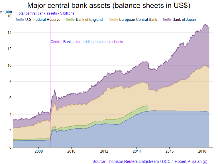
The grand-daddy of systemic liquidity is, of course, the aggregate stimulus provided by the leading global central banks (the Federal Reserve, European Central Bank, Bank of Japan, People’s Bank of China, and Swiss National Bank – CB5). Their aggregate balance sheets have been feeding economies and financial markets since late 2008 (see graph above).
After the US Federal Reserve launched its Quantitative Easing programs in November 2008, major global central banks followed suit. The volume of the global bank reserves generated by those large-scale asset procurements were so large that for all intents and purposes those reserves have become the global Monetary Base (NASDAQ:MB) of the global central banks (CB5). The aggregate global Monetary Base has been credited with pushing up the valuation of equity and other asset markets around the world. We also credit the aggregate global MB for uplifting US and global growth.
Systemic liquidity's impact on US GDP growth
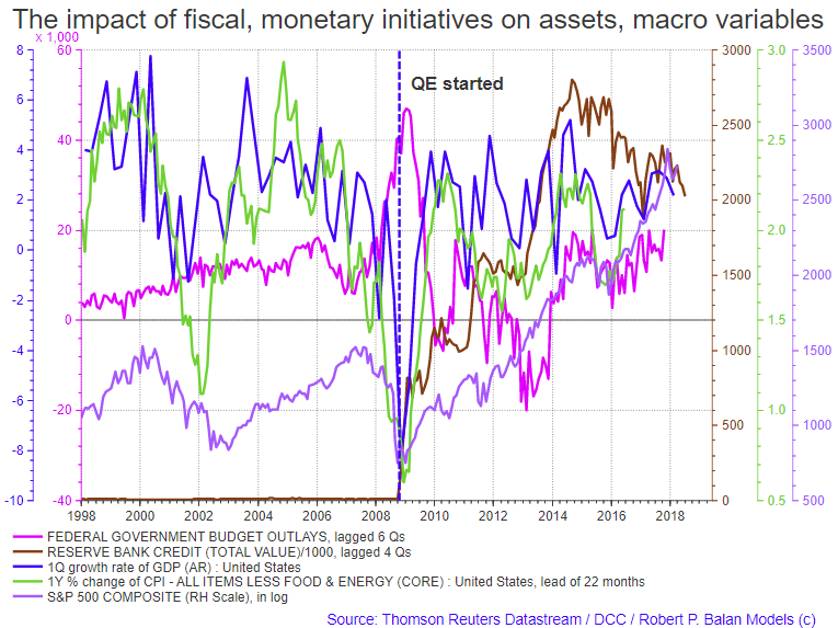
The conventional wisdom being foisted by some academics is that the global monetary stimulus from the central banks' large-scale asset procurement did wonders for financial markets but did little or nothing to improve domestic economies, or for that matter, world GDP growth. That is actually a misrepresentation of the positive impact those large-scale asset purchases have on the US and the global economy, which was extensive (see graphs above, and two graphs below).

As these central bank balance sheets have subsumed, and have become the de facto global Monetary Bases, these vectors have become important drivers of economic growth, through linkages with growth in bank loans and investments (see graph below).
US GDP growth is very sensitive to the fluctuations of the flows of the Fed's Balance Sheet, Total Bank Reserves at the Fed, and Total US Deposits. And the growth of bank deposits (loans + investments = deposits, not the other way around), can be largely accounted for by the expansion or contraction of Federal Reserve bank credit. The Fed's balance sheet and aggregate bank reserves at the Fed lead Total US Deposits (loans+investment) by 2 months (see graph below).
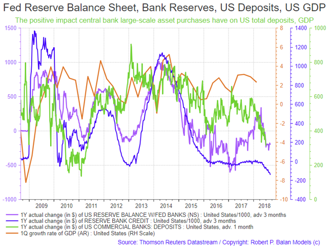
Providing ill portents, deposits have been plunging since November 2017 – and the bill will soon come due. Liquidity flows from these vectors have been leading changes in US growth by a quarter. And the sharp decline in global Monetary Base since March last year does not bode well for continued or sustained uptrend in US GDP growth after Q3 2018 (see graph above).
Systemic liquidity from fiscal expenditures
We have been working on this thread for some time, as part of our long-term "scan" of systemic liquidity -- the very long-term variety. That's why were intrigued by the latest forecasts of the US Congressional Budget Office (CBO). The CBO laid in detail the dynamics that could lead to a sharp growth slowdown as from late 2018 to 2020 (see graph below). Look closely into the CBO forecasts of government outlays and in discretionary spending, which are due to fall until 2020 (see graph below).
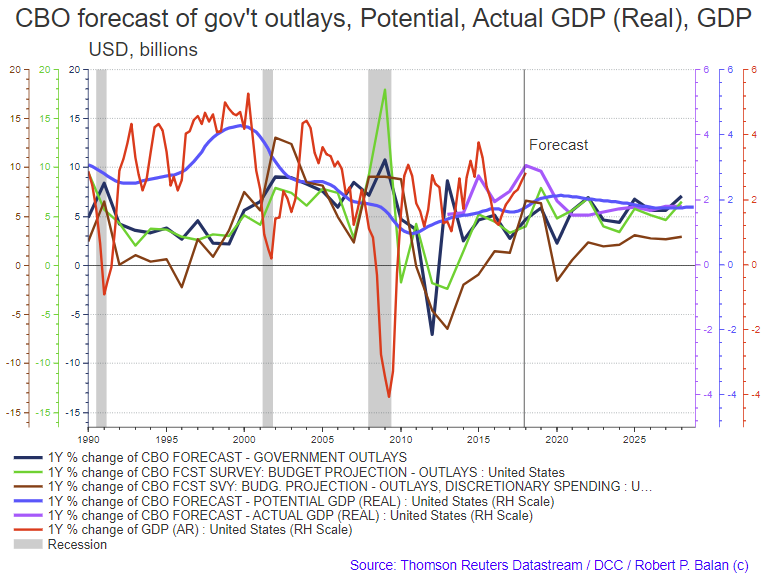
What is especially relevant and telling in our opinion is the sharp decline in fiscal discretionary spending from late 2018 to 2020 (black dotted line, see graph below). It resonates with us because the changes in this data lead the changes in GDP and the changes in risk asset prices. The sharp fall in fiscal discretionary spending after 2018, along with the expiration of tax relief by late 2018, could lead to growth recession in 2019-2020. That could bring down the price of risk assets (see graph below).
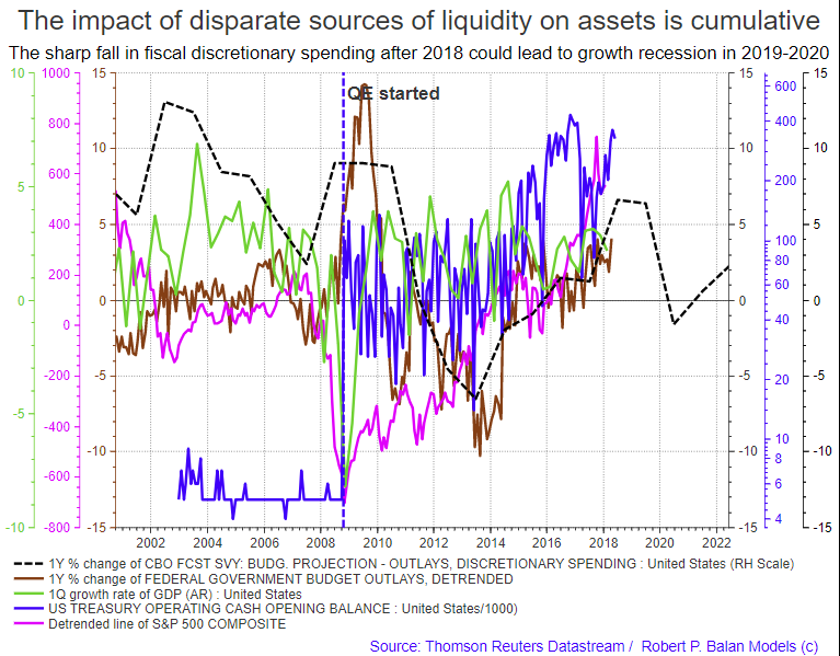
A monetary policy tightening in the entirety of 2018, and fiscal consolidation by late 2018, extending into 2019-2020, are scary prospects, as they would be happening at the same time. The withdrawal of systemic liquidity from those policy actions will have adverse consequences on risk assets. Nonetheless, there is still time to benefit from the recent upwelling of growth worldwide as the spill-over effects would still flow into risk assets over the next 2 quarters.
Systemic liquidity's impact on financial markets
After the US Federal Reserve launched its Quantitative Easing programs, major global central banks followed suit. The volume of the global bank reserves generated by those large-scale asset procurements were so large that for all intents and purposes those reserves have become the Monetary Base of the central banks of the US, the EU, Japan, China and the Switzerland (CB5). The aggregate global central bank balance sheet has been credited with pushing up the valuation of equity and other asset markets around the world.
The impact of those aggregate global reserves on financial assets was, and is, enormous. During the time global central banks were adding to their balance sheets, financial assets have become beholden to the flow of that global aggregate systemic liquidity. The prices of financial assets have risen as the flow of the aggregate Monetary Base rose, and opposite is also true. This is especially true of the US stock market and US bond markets (see graph below).
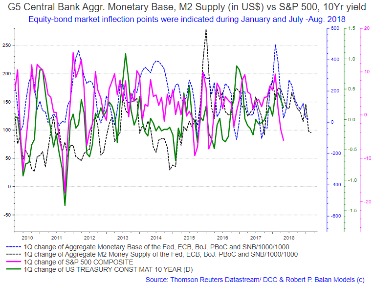
In the graph provided above, for 2018, the flows peaked in January, which coincided with the peak in the S&P 500 Composite, and in the 10-year US Treasury Bond Yield. There is another peak in the liquidity flow being shown in July – August, this year. We therefore expect financial assets, especially equities, to make significant peaks at that time (see also graph below).
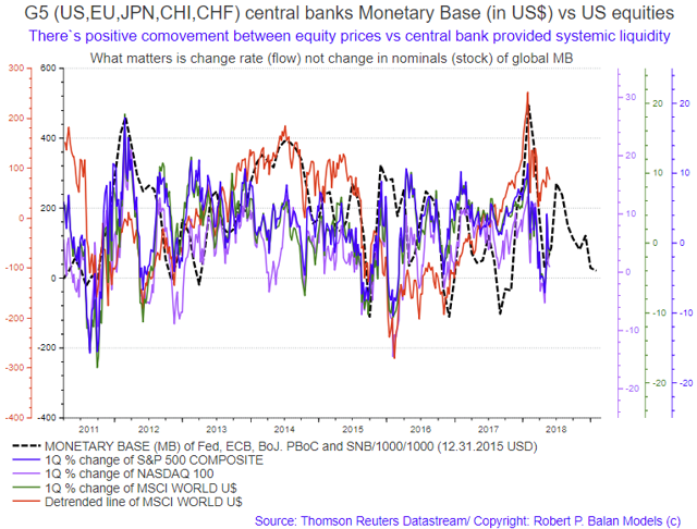
The impact of the CB5’s balance sheets (and Monetary Bases) were not confined to equities and bond yields – the US dollar, as the world’s transaction and reserve currency, is also impacted by flows in global systemic liquidity via the Quantity Theory of Money (QTM). In monetary economics, QTM states that the general price level of goods and services is directly proportional to the amount of money in circulation, or money supply. This general theorem also applies to the inverse value of the US Dollar (with DXY as proxy – which incidentally provides the link between inflation and the US Dollar). The more global liquidity (represented by the CB5’s aggregate Monetary Base) there is, the weaker the US Dollar, and vice versa (see graph below).
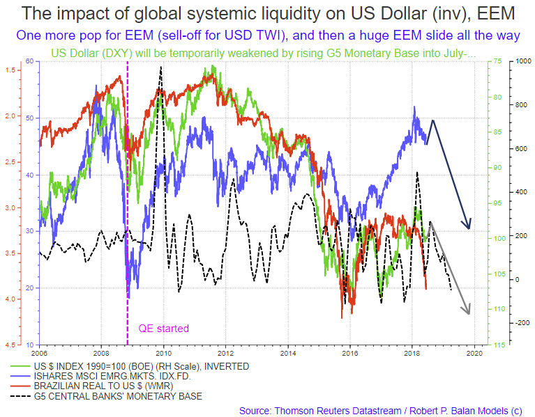
The course of the US Dollar has a very significant inverse impact on Emerging Market economies and currencies – as the USD strengthens, the EEM and EM currencies weaken proportionately. This was and is especially true after QE programs became world-wide. The outlook for the DXY based on this relationship: the DXY should weaken going into July-August this year but will massively appreciate in value at least until late Q1 2019 (see graph above).
The outlook for global systemic liquidity from here
To some extent, that inflow of liquidity is still flowing in, especially from the European Central Bank (until year-end 2018), the Bank of Japan, and to a more limited extent, the Swiss National Bank.
There is a long, distributed lag between those liquidity flows and its direct impact on the financial assets, which is usually from 11 to 12 months long. Put another way, the systemic liquidity flows in these aggregates today will show their maximum impact on the prices of asset prices 11 to 12 months from now.
We have added the aggregate M2 money supply of the 5 central banks (in terms of US Dollars) as a control variable and is also lagged 12 months. The global aggregate M2 money supply control variable tends to peak or bottom in concert with the global Monetary Base aggregate. This system of having control variables is a very important part in making sure that we are not looking at spurious correlations. Having two different aggregates in the same monetary set confirming each other's move provides a reasonable check and balance on any conclusions we will make.
This is how this tool is used in a trading environment
As explained in the April 2018 edition of the Capital Observer, in our experience, the most reliable correlations (relatively speaking) can be found between the causality from monetary flows (changes in systemic liquidity) to subsequent changes in asset prices. That's why we rate this tool with high confidence to be used to help for the timing of the trades -- from stimuli to peak impact on the price.
In that April 2018 Capital Observer article (April 13, 2018), we showed the impact that systemic liquidity can have on the price structure of many key assets. We provided general descriptions of expected market action over the next few weeks and months based on liquidity developments from the US Treasury and the Federal Reserve. Specifically, we said: "Expect a small recovery, probably for a week - a significant decline follows thereafter. But we should see a cyclic low sometime in late April-early May, followed by a new upside phase of the bull market.”
The US equity markets bottomed in May 3, 2018.
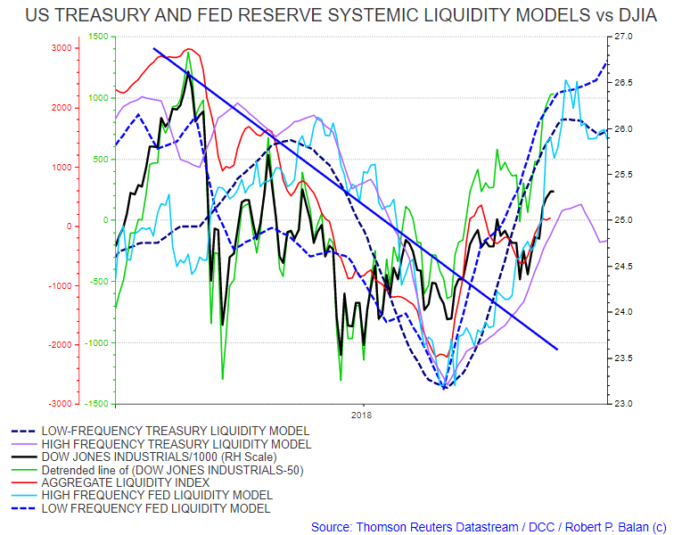
For bond yields, we said: “Expect a further decline for a week – an uptick in yield follows thereafter. But we should see a cyclic high sometime in July, followed by another downtick in yields (see chart above).
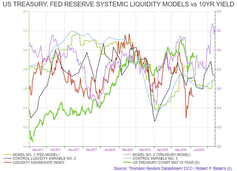
Very often, it is the change rates in the nominal values (flows), not the absolute changes in nominal value (the stock), which display the best comovements (or correlations, if you may). Note, however, that the response of asset prices to the impact of those flows is variable; some assets respond more quickly to the flows; for other assets, the impact of those flows come later.
Nonetheless, despite the variance in response, the individual distributed lag between monetary stimulus and the point of maximum impact it has on a specific asset price can be very consistent over long periods. This is how these tools become useful -- the liquidity flows become the leading directional indicator of risk assets, with forward-look of several months, even up to several years in some cases -- the consistency provides reliability.
There are several sources of systemic liquidity, and those sources do not necessarily synchronize their activities. While there are elements of seasonality in the liquidity mix, sometimes, there are episodic variations which could skew well-established patterns which have held up for years. Usually, the well-established patterns come back after a few errant cycles.
The key to a successful use of systemic liquidity as bedrock in the analysis of risk asset price dynamics lies in being able to corral that variability into a singular vector which could relate to the behaviour of risk asset price. One way to handle the chaos and to make the math work more tractable is to index the data, then find a calibrated match of the resulting vector versus the regressed price of the asset in the time continuum.
I published a significant amount of background materials on systemic liquidity in this recent Seeking Alpha article. This article provides more details which cannot be accommodated in current piece.
Summary:
So now, we have a general understanding of what has driven the markets in the past. We also now understand that a change in the systemic liquidity flows which is being provided by the large global central banks today will show its maximum impact 11 to 12 months in asset prices thereafter.
Although the Federal Reserve has stopped providing Monetary Base liquidity via its balance sheet, the European Central Bank and the Bank of Japan are still providing global systemic liquidity and the ECB said they will do so will year-end.
However, we now also understand that this resource is winding down, and in fact, after a favorable uplift into July and August, the flows start to die down, and that will have adverse impact on the prices of financial assets going into Q4 2018 and beyond.
Nonetheless, the next few months are still good time to invest in risk assets - we may be looking at this period with fond memories during the 2019-2020 blah period. Take advantage of the run up into Q4 2018 when the tax exemptions are at their maximum. But do not overstay - take profits late in the year. We will discuss these issues again when it is time to exit the markets.
The global economy is also at risk if the Fed follows through on its rate hike regime of two, possibly three more, this year. Along with a strong US Dollar, the Fed's monetary policy course, which was reaffirmed by Chair Jerome Powell in this week's FOMC meeting, has the power to devastate large swaths of the Emerging Markets. This is a theme that has been thoroughly discussed in previous issues of the Capital Observer, so there’s no further need to go into more detail at this time. The risks were also discussed in this recent Seeking Alpha article. Those publications show that the economy (US and global) and the financial markets are facing a triple whammy after Q3 this year, which will likely lead to lower asset prices and more subdued growth in 2019.

Comments
Log in or sign up to join the conversation.