Primer: Dynamic Option Hedging

This article attempts to provide a non-mathematical explanation of dynamic option hedging. Although the original reasoning to dive into this topic was the hedging of options on interest rate products, for simplicity, it will discuss an equity option on the basis that more people are somewhat familiar with stocks and stock options. It may even be of use to readers who are in similar position the author was in when he entered into finance: mathematical background, but little knowledge of finance. It is possible to plunge into the mathematics of financial derivatives1 without having an intuition for why they behave the way that they do, but that intuition is needed to grasp how they fit into the financial system.

Options

An option can either be traded on an exchange or as an “over-the-counter” legal contract traded between two counterparties. The most basic class of options are the ones considered here, which give the counterparty that “owns the option” the option to buy or sell a specific underlying security at a fixed price on a fixed date in the future (with the counter-party being the party that is selling/buying, it has “sold the option”). Since it is an option, the owner can just let the option expire (presumably because the transaction is not profitable).

There are therefore a few key parameters that determine the value of the option, that are fixed in the contract definition.

• Is it an option to buy or sell the security? In equities, the options to buy are termed “calls,” while the option to sell is a “put.” The same terminology holds for fixed income exchange-traded options, but the terminology is wackier for options on swaps.

• At what price is the transaction to buy/sell taking place at? This is known as the “strike.”

• At what date does the option expire, which is the last (or only) date the owner of the option can make the transaction. Since the contract has no enforceable terms after that date, the option is then worthless. (Technical note: there is an extra parameter that I attempted to absorb into a single mangled sentence — is it possible to exercise the option ahead of expiry? We are going to ignore that possibility, since we are not pricing the option.)

In order to avoid using too much jargon, I will stick with one option configuration in this text. The parameters are as follows. The owner of the option has the right to buy 1 share of a company2 at a date in the future (e.g., 3 months from now) at the price of $100. This is therefore a call option. The “date in the future” is vague since I will not be discussing the value of the option, and all that matters for our purposes is that it is not about to immediately expire. We will assume that the current price of the share is around $100. We will also assume that the stock will not pay any dividends ahead of expiry.

(Background comment. This call option is ultimately more valuable if the price goes up. It matches the stock options given as incentives to employees. It also aligns with the option to prepay a mortgage. The borrower in a mortgage is “short” the debt (has a negative position). The option to prepay allows them to buy back the mortgage debt that owe at a fixed price. Going the other way, a put option benefits from the price falling. They correspond to owning insurance on an equity position.)

Jargon note: It was very difficult to write this article without using the jargon terms “long” and “short.” If you are long something — an equity, or an option — you own it. If you are short it, you have sold it and have a “negative position.” E.g., if you are short one share of the company, you are in the financial equivalent of owning -1 shares. I am also just going to write that we “buy” or “sell” the option, which sort-of works for exchange-traded options, but many options are contracts between two counterparties, so that terminology is stretched.

Valuation of the option is easy at expiry (last time the option can be exercised):

• If the price of the equity > $100, then the value of the option is equal to (stock price) - $100. For example, if the stock price is $101, the option is worth $1. We can buy the option for $1, exercise the option by paying $100, and end up with an equity worth $101 (equal to the outlay). If the stock price is $102, the option is worth $2, etc.

• If the price is less than or equal $100, the option is worthless — you can buy the equity cheaper (or at the same price) in the market instead of exercising.

The figure below shows this value at payoff graphically. The top panel shows the profits on owning the option, and the profit function consists of two line segments.

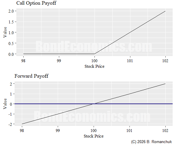
The bottom panel shows the profits on either purchasing the stock at $100 or entering into a forward contract to buy one share at $100. If the price ends up at $100, the position breaks even ($0 profit). Otherwise, the profits are a linear function (around the $100 point), with profits increasing as the price goes up, and losses if the price drops below $100.

The distinction between the two instruments is driven by the shape of the profit/loss line. The simple “buy the equity”/”buy the equity forward” strategy has a payoff that is a line, with both profits and losses. The option payoff is piecewise linear3 (which is a subclass of nonlinear functions), and is such that the option cannot end up with a negative value. (You can lose money buying options, but the loss comes from buying them at a higher price than what they expire at.)

The linear/nonlinear payoff distinction made its way into fixed income jargon, where instruments with options were “nonlinear” (such as mortgages with prepayment options) and those without are “linear” (most bonds, swaps, bond futures, etc.) Using this jargon, we are going to be discussing hedging nonlinear instruments with linear ones (which are more widely traded).

Option Valuation

Option-like securities (warrants) had been traded for a long time, even though straight options were ruled out regulations. Based on discussions with senior professors back when I was in control systems academia, people were leaving mathematical fields like control systems to make money trading warrants even in the mid-1960s. At that time, it was a bit of a black art, without “textbook” solutions. However, the Black-Scholes pricing formula arrived in 1973, along with deregulation that allowed trading in options.

The key insight to the Black-Scholes formula — which was not really clear to me when I first picked up The Mathematics of Financial Derivatives by Wilmot, Howison, and Dewynne — is that the value of an option is equal to the expected profits of hedging the option until expiry (where “expected profit” is the mathematical meaning). (The previously-mentioned textbook is the most straightforward option-pricing text that I am familiar with that goes into the mathematics.) Going the other way, the value of selling the option is equal to the expected hedging losses on that position. Although my intuition was that the value would be driven by the probability distribution at expiry, the hedging value is of more importance to financial market participants.

Why Hedge?

Before discussing how hedging works, let us look at why one hedges in the first place. In our example call option, the most natural story is the considerations of a market maker.

A market maker is a market participant that puts themselves in between others. They “make a market” by posting bid and ask prices — prices at which they are willing to buy (or sell) the instrument. If you want to survive as a market maker, you need to make your bid price less than your ask. Your profits are supposed to be made by earning the bid/ask spread. (You also hear bid/offer instead of bid/ask, but I believe bid/ask is preferred in equities and so is heard more often.) For example, say your bid/ask on a security is $99.50/$100.50 (which is pretty honking wide). If someone sells you the security and you can resell it immediately, you will net a $1 round-trip profit (you buy at $99.50, sell at $100.50) over a short time interval. Everyone else faces “transaction costs” associated with the bid/ask spread, that is how the market maker is supposed to make money (not by betting on the prices of the securities).

The problem is that you cannot ensure that you have clients that magically pop up to make trades that instantly close your position, you will end up stuck with inventory (or a “book”). The skill of market making is adjusting your bid/ask prices so that you keep your book balanced.

Returning to our example, imagine you are a market maker where some client sold you the call option just ahead of the market close. Although you liked the business, you are unlikely to close out the position with someone else buying it from you before the close. And you do not want to be stuck with the position before you leave for the weekend. (Yes, a $100 option position is too small to care about, but just add zeros to the position size so that the risk is more plausible.) Since you are a market maker, you do not want to go to another market maker to close the position (since you are eating the transaction cost). Instead, you dig out your options textbook and re-read the chapter on dynamic hedging.

Dynamic Hedging Without Maths

The secret to dynamic hedging options with “linear” instruments is the hedging ratio (often called the “delta”), or the price sensitivity of the instrument. In fixed income, we often to refer to the “DV01” — “the dollar value of one basis point.” That is, how much does the value of an instrument or portfolio change if we have a one basis point (0.01%) shock to the interest rate curve? Since this is an equity option, we are not interested in the interest rate sensitivity, we are interested in how much the value of the option changes if the price of the underlying equity changes (either in percentage terms, or absolute)?

Although we consult the Black-Scholes formula to get this sensitivity, we live in 2026 and use digital computers. We instead consult our portfolio analysis software, which spits out the hedging ratio.

In our case, we will assume that the hedging ratio is exactly 0.5 (which is what happens when the stock price is very near the strike price of $100). That is, the option value will have a price shock that is equal to 50% of the price shock change of the equity for small price changes. For example, if the equity rises by $0.02 (e.g., from $100 to $100.02), then the call option rises in value by $0.01 “all else equal”. But if the equity drops by $0.02, then the value of the option drops by $0.01.

We need to immediately address the “all else equal” part of the statement. There are multiple parameters that are input into the Black-Scholes formula to give the option value. We are assuming that all the other parameters are unchanged in this exercise. (Certain parameters — like the expiry date and the strike — are fixed in the contract, so they cannot change for this option.) The most important “other variable” is the so-called implied volatility — which I will return to below. Raising (lowering) the implied volatility will raise (lower) the price of the option, even if the price of the equity is unchanged. However, we cannot hedge the implied volatility with linear instruments — all we can hedge is the effect of price changes in the underlying instrument.

So what we ultimately do to hedge our long call equity option position (which is on one share) is to sell short 0.5 shares of the equity and call it a day. (To repeat the definition of short sales, this means that you end up with the equivalent of owning -0.5 shares.) The interpretation is straightforward: the call option benefits from the price rising, but the short sale loses money in that case. Since the call option has half the price sensitivity of the short sale, the short sale has half the notional position size.

What If Prices Move?

The price sensitivity measure we calculated were for very small movements. What happens if the price moves appreciably?

Let us say when we get back to the office, and the price of the equity jumped to $101. Our call option position will have risen in value (assuming unchanged implied volatility), but we lost money on the short equity position. If implied volatility was indeed stable, the two positions should have had largely cancelling profits and losses. The dynamic hedging eliminates (most of) the effect of the stock price change.

However, when we re-run our portfolio sensitivity analysis, we discover something troubling. The sensitivity of the short position is roughly constant, but the price sensitivity of the option rose. (I am not going to supply a number because I am lazy.) The sensitivity of option and short position no longer cancel out, so the position now gains (loses) money if the underlying stock price rises (falls). Since we are market makers and not stock speculators, this is unwelcome. So we need to sell short more equity to balance out the option. (The maximum sensitivity of the call option is 1, so the most we could end up shorting is just under 1 share.)

Now that we are hedged again, we go back to doing whatever market makers do all day. Then imagine we are stuck with the option position overnight again.

We discover the next day that the stock round-tripped back to close to $100. Once again, the sensitivity of the option is 0.5. But since we sold short some of the equity to bring back the net exposure to zero when it was at $101, we are now over-hedged (too large a short position). So we need to buy back the amount we bought earlier at $100 to bring the short position to being 0.5 shares.

Although the hedge is back in place, we now can note something. We were forced to sell short a small amount of the equity at $101 to hedge our option position. We then had to buy back that short sale at $100. Since we sold at a higher price than we bought, we made money on that adding and subtracting that extra hedging position.

More generally, we will see this pattern of behaviour if the price is jumping up and down, even if it does not conveniently return to its exact starting point. The hedging transactions generated by hedging a long option position are “counter-trend” moves that end up being profitable if price moves revert back-and-forth.

In an idealised probability setting, the expected profits from hedging will be driven by the “random noise” implied by the second moment of the probability distribution (which the standard deviation (or “sigma”) measures over a sample).4

Hedging a short position in an option is the reverse of the above. If we were short the call option, we then would have had to use a long position in the equity hedge the short option position. When the price went to $101, we would have had to buy to rebalance our hedging ratio. We would then have had to sell at $100 when we rebalanced again — eating a loss.

“Long (Short) Volatility”

The “directional hedge” discussed above (largely) removes the risk associated with the underlying equity changing price. However, the long position in an option is not risk-free: we will instantly gain (lose) money on the option if the implied volatility rises (falls). Our portfolio analysis software will spit out an explanation: there are more risk factors than just the underlying price change. By owning an option, we have direct exposure to the implied volatility (which is a measure of how expensive options are).

Since we make money if implied volatility goes up, we are “long volatility.” (We would be short volatility if the opposite were the case.) Linear instruments have no exposure to the implied volatility, so they cannot be used to hedge volatility risk. The only way to hedge that risk is trading other options, or wacky derivatives like volatility swaps.

There are other risk factors as well, but they are usually second order effects. The value of options decay as they get closer to expiry, so a long option position has a steady “time value” (“theta”) that eats away at its value. Interest rate derivatives with long expiries (like a prepay option 10 years in the future) are harder to model because the value of the option on exercise needs to be discounted by the interest rate — while interest rates are also the underlying instrument. (This is why you do not want to start with fixed income options if you are learning about options.)

Macro Effect of Hedging

Although hedging by itself is not that exciting, if everyone is doing it in the same direction, we can have problems. In particular, if we have a lot of entities with short option positions attempting to hedge them at the same time, they are forced to act in a pro-cyclic fashion: if the price rises, they need to buy more, while they are forced to sell more if prices fall.

In the equity world, problems would occur if a whole bunch of people were stupid enough to sell “portfolio insurance” and try to dynamically hedge their positions at the same time. (Whoops, what happened in 1987?) In the fixed income world, the structure of conventional mortgages means that mortgage issuers are selling prepayment options in incredibly large size to homeowners, and some poor devils attempt to hedge a portion of that position.

Concluding Remark

Option mathematics is complicated and annoying. But if we are managing a portfolio and not a quant developing pricing algorithms, we can just use portfolio analysis software to see the numeric sensitivity of our portfolio to risk factors (like stock prices rising). We can hedge out the “directional risk” of options using instruments without options embedded in them, but we will have to continuously adjust our hedging ratio. We will lose money from those adjustments if we are short options (but we hoped to have covered that from the money we got from selling the options).

1 The term financial derivative has nothing to do with the use of derivative in calculus. The term refers to instruments whose value derives from having contractual claims on an underlying instrument. For example, a bond future derives its value from bond futures ultimately being a claim on some underlying “cash” bond based on the futures specification. Options are the most interesting (and complex) member of the class of derivatives.

2 Exchange-traded options are normally board-lot sized (100 shares), but I am using one share to keep numbers simple.

3 My academic work ended up specialising in the analysis of piecewise linear systems, so this is of sentimental value to me.

4 There’s a certain amount of internet experts who sneer at the standard deviation and cackle at “sigma.” Yes, the Black-Scholes is not a perfect description of option pricing, but it is close enough that it (and its variants) are used as the option quotation benchmark. The main effect of imperfections is that implied volatility is not flat across strikes and expiries.