Have You Stress-Tested Your Portfolio Strategy?

The world is awash with backtests that lay claim to new portfolio techniques that provide superior results for managing risk, juicing return, or both. What’s often missing is a robust stress test to confirm that the good news is more than a statistical anomaly. Crunching the numbers on a single run of history that looks encouraging is one thing; taking the backtest to the next level by simulating results across a range of alternative scenarios as a proxy for kicking the tires on the future is something else entirely. Not surprisingly, only a tiny sliver of the strategies that look good on paper can survive this higher standard. That’s a problem if you’re intent on publishing a regular stream of upbeat research reports that appear to open the door to money-management glory. But for investors wary of committing real money to new and largely untested portfolio strategies, stress testing is critical for separating the wheat from the chaff.

As a simple example, let’s review the results for a widely respected tactical asset allocation strategy that was originally outlined by Meb Faber in “A Quantitative Approach to Tactical Asset Allocation.” The original 2007 paper studied a simple system of using moving averages across asset classes to manage risk. The impressive results are generated by a model that compares the current end-of-month price to a 10-month average. If the end-of-month price is above the 10-month average, buy or continue to hold the asset. Otherwise, sell or hold cash for the asset’s share of the portfolio. The result? A remarkably strong return for what we’ll refer to as the Faber strategy over decades, in both absolute and risk-adjusted terms, vs. buying and holding the same mix of assets.

For illustrative purposes, let’s re-run the data with just two ETFs—a simple 60%/40% US stock/bond mix based on a pair of ETFs: SPDR S&P 500 ETF (SPY) and iShares 7-10 Year Treasury Bond (IEF) for a sample period that runs from the end of 2003 through the present. As the chart below shows, the Faber strategy looks quite impressive vs. a buy-and-hold portfolio that sets the initial weights to 60%/40% and leaves the rest to Mr. Market.

So far, so good. The Faber strategy performs in line with the results in the original study. Applying tactical asset allocation by way of the paper generated less volatile results with a moderately higher return over the sample period. The annualized Sharpe ratio (a risk metric that adjusts return based on volatility) for this version of the Faber strategy over the 2003-2016 period is 0.87. That’s a solid premium over the buy-and-hold’s Sharpe ratio of 0.60. Taken at face value, the higher Sharpe ratio tells us that the Faber strategy is superior even after adjusting for risk (return volatility).

But let’s take this up a notch and run a Monte Carlo analysis on the Faber strategy. The plan is to re-run the strategy multiple times and collect the results. In other words, we’re going to simulate alternative histories for a deeper read on what the future might bring. Rather than rely on one backtest, albeit one based on actual history, this technique allows us to consider how the Faber strategy might perform if history could be repeated thousands of times with different results.

The heavy lifting for running the Monte Carlo test will be performed in R. The key piece of code is the sample() command. By resampling the Faber strategy’s actual returns we can produce alternative outcomes—10,000 outcomes in the case of this test.

The box plot below summarizes the output in terms of the range of annualized Sharpe ratios for the 10,000 simulated runs. Note the red box, which marks the 0.87 Sharpe ratio in the original backtest using actual data. But this result looks quite high in the context of the simulated data. The implication: the original backtest outlined above may have oversold the strategy’s results in terms of what we can expect going forward with the out-of-sample performance.

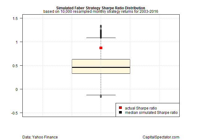
Indeed, the original 0.87 Sharpe ratio is well above the median Sharpe ratio of 0.46 for the simulated data and the 0.63 SR at the upper level of the interquartile range (the 75th percentile). The results don’t necessarily invalidate the Faber strategy, but the elevated Sharpe ratio in the original test suggests that the sample period (2003-2016) may have been an unusually fertile period that isn’t likely to deliver a repeat performance any time soon if ever.

In short, it appears that we should manage expectations down relative to the original backtest. In turn, the stress test could be the basis for revising the strategy or turning to another methodology for managing money.

To be fair, a robust stress test would run a series of analytics beyond Sharpe ratio simulations. But this toy example is still a powerful reminder that first impressions with backtests can be misleading and, in the worst cases, hazardous to your wealth.

The challenge is developing reasonable expectations and all too often backtesting procedures fall short. Keep in mind too that there’s a reason you’ll really find a backtest that highlights poor results: research that reveals failure tends to be buried.

The good news is that there’s a spectrum a techniques (see here, here and here, for instance) for deciding if the initial results of an encouraging backtest have a reasonable chance to hold up in the real world going forward. To be fair, the Faber strategy overall has been tested extensively by analysts and continues to offer upbeat results, albeit with all the standard caveats. But that’s the exception to the rule.

It’s a safe assumption that most backtests in the grand scheme of research efforts that see the light of day will fail to deliver anything close to the stellar results outlined. Fortunately, a multi-faceted stress test can go a long way in reducing the risk that the research du jour is leading you astray.