


Sixteen years of above-average returns came mostly from rising valuations, and that is the one source that cannot be repeated from here.
Key Takeaways
Since the end of 2009, the S&P 500 compounded at 14.34% a year, or 11.41% after inflation. The long-run real average since 1881 is 6.72%.
Of that 11.41%, some 4.33 points a year came from nothing but the valuation multiple doubling.
Across 146 years, 140 of the 164 starting months with a CAPE of 25 or higher produced a below-average next decade. The 24 exceptions all fall in 2014 to 2016.
The highest CAPE ever to precede a decade this good was 26.95, in August 2016. Today’s reading is 41.04.
In 2016, McKinsey warned that the “golden era” for investors had ended. Falling rates, fatter margins, and a rising multiple had done their work in creating above-average returns. Younger savers, the report said, would have to work seven more years or save nearly twice as much. Ben Carlson went back and graded that call this month. Since that spring, U.S. stocks have returned roughly 15% a year and more than tripled, European shares compounded near 10%, and a saver who took the advice and doubled their contributions now has a very comfortable problem. The call was wrong. Carlson’s verdict is blunt and correct. Sometimes the three most useful words in this business are “I don’t know.”
“Strip the multiple out and the last sixteen years were ordinary. Every point of excess came from investors agreeing to pay more for the same dollar of profit.”
I also have to take that same hit, as I have previously published my own versions of that caution, and the market ran anyway. Anybody claiming they called the last sixteen years of above-average returns is selling something.
Where The Above-Average Returns Actually Came From
While the bulls certainly have control of the narrative, there is a problem with treating that scoreboard as the end of the argument. The bears weren’t wrong about the inputs. They were wrong about ONE variable. Which one matters is important because it will decide whether the case still stands today.
Let’s start with the data. I pulled Robert Shiller’s monthly series back to 1871 and broke real returns down into their specific components. Real total return splits into three pieces. What earnings were, what dividends were paid out, and what investors decided those earnings were worth.
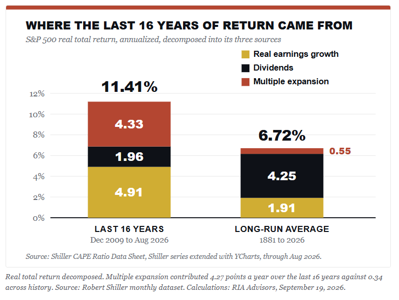
Real earnings grew 4.91% a year. That’s close to three times the 1.91% long-run rate. Dividends chipped in 1.96 points against a past norm of 4.25, because yields today are far thinner. Then there’s the third bar. The CAPE ratio climbed from 20.32 at the end of 2009 to 41.04 in October, and that single “re-rating” of the same earnings stream, with no help at all from profits or payouts, added 4.33 points a year to what investors took home. Look at how much of the left bar it is.
Strip the multiple out and the last sixteen years delivered roughly 7% real, which is almost exactly the long-run average. Every point of excess came from investors agreeing to pay more per dollar of smoothed profit. Such is the anatomy of a “golden era.”
That’s the piece McKinsey missed. They had the right list of tailwinds, but they just assumed the “re-rating” had finished. But it hadn’t, and it ran for another decade, producing the above-average returns that made the forecast look foolish.
Why Above Average Returns Can’t Repeat From Here
Now run the same math forward. The multiple would have to add another 4.33 points a year for sixteen years. That takes a CAPE north of 83. Not 41. Eighty-three. No market on record has held half that.
Which raises the question that the decomposition doesn’t answer. What drove the first doubling?
The discount rate did most of the work. Roughly half those sixteen years were spent with the funds rate pinned at zero, from January 2010 through December 2015 and again from March 2020 into 2022. The 10-year average yield was 2.20% from 2010 to 2021, compared with 4.71% for the entire Shiller record since 1871.
The Fed’s balance sheet went from under a trillion dollars to a peak near $9 trillion. Argue all you like about whether the Fed led that or followed it. Either way, money was cheaper for longer than at any point on record, and cheap money lifts what buyers will pay per dollar of earnings while quietly flattering earnings themselves.
Here’s the trap in that. The only thing that brings ZIRP and QE back is the crisis that justifies them. Either rates hold near 5%, and the multiple gets no help, or something breaks badly enough to put the Fed back at zero, which means the damage already happened. Baa corporates yield 6.47% today, and the maturity wall refinances at the new number, not the old one.
Going back to the Shiller data set, I tested every month from 1881 onward. For each one, I logged the CAPE, then the real total return over the next ten years. That gives 1,628 overlapping readings. They stop in August 2016, because any month after that doesn’t have ten years behind it yet.
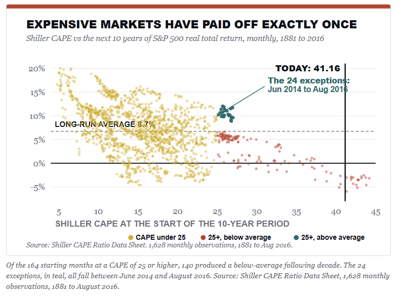
The pattern isn’t subtle. Of the 164 starting months with a CAPE at or above 25, some 140 of them, roughly 85%, gave back a decade below the 6.72% long-run average. Go higher, and it gets worse. The 57 months above a CAPE of 30 averaged a loss of 1.02% per year, and the best of them posted a gain of 4.49%.
Before we proceed, we must discuss the caveat, because somebody will raise it, and they’re right to. Two dozen of those expensive months beat the average. They ran from June 2014 through August 2016, starting CAPEs between 25.16 and 27.00, and delivered real returns of 8.86% to 12.02% over the decade that followed. So an expensive market has paid off. Exactly once.
Look at what that particular decade contained. It caught the back half of ZIRP, the 2020 emergency response, and the AI earnings expansion, and it finished with the CAPE at 41 instead of 26. The one time in 146 years that a high starting valuation was paid, it paid because the multiple expanded again from an already expensive base. That is the engine described above, and it’s the engine that is most likely not returning anytime soon.
The overlap caveat matters a lot. When looking at those 1,628 readings, they were not 1,628 independent events. This is because the ten-year windows overlap, and the months within one episode repeat the same story. For example, the “expensive” months cluster into four episodes: 1901, 1928 through 1930, the long stretch from 1995 to 2007, and 2014 to 2016. Three ended badly. One didn’t.
So call it three out of four, not 140 out of 164, and the honest reading is that expensive markets usually disappoint and occasionally don’t.
26.95
The highest starting CAPE ever to precede a decade as good as the one we just had. August 2016. Today we sit at 41.04.
Even the exception started from a valuation of 27, and it needed the multiple to run to 41 to get there. We’re now being asked to believe the market can do it again from 41. Such is the “this time is different” bet, whether or not anyone phrases it that way.
“The bears had the right list of tailwinds. They simply assumed the re-rating had finished. It hadn’t.”
The Bullish Case Against The Next Secular Bear
While the data is clear, the bulls do have a serious answer to all of this.
The bullish argument is that above-average returns may remain for three primary reasons:
The current CAPE ratio of 41 is a broken yardstick, because the measure still drags the 2020 earnings collapse into its ten-year average.
It ignores the shift from capital-heavy industry to software margins, and accounting rules expense the very intangible spending that builds those fat margins.
Corporate buybacks also changed the cash math. A 2% “yield” in 2026 isn’t the same as a 2% yield in 1962.
Every one of those points is fair. It’s why real earnings grew at triple the old rate instead of reverting. I can’t argue the AI capital cycle is a fiction either. The spending is REAL, and the profits so far are real.
Then there’s the bull’s best evidence, which happens to be mine too. The Fed raised the Fed funds rate from zero to more than 5% starting in 2022, and the CAPE promptly fell from 38.30 to 27.08, exactly as the discount-rate story would predict. Since then, that valuation multiple has climbed to 40.94 anyway, with the 10-year at 5.01%. The multiple rose into the most aggressive tightening in forty years.
The obvious answer is uncomfortable for both bulls and bears. A multiple that expands while the discount rate rises isn’t resting on rates at all. It’s resting entirely on what investors believe earnings will do, and today those estimates are very exuberant, as we noted recently.
“Corporate earnings just broke above a trend that had contained them for more than 90 years.”
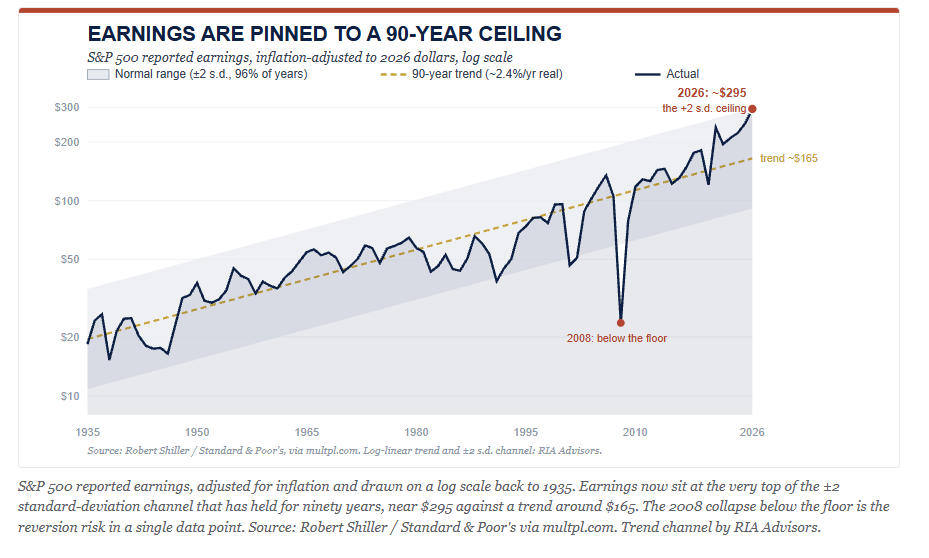
With expectations as high as they are currently, that foundation is much more fragile than a rate-supported multiple. If the earnings story disappoints, there is nothing sitting below the market to support it.
Here is where it gets interesting. Grant the whole case. Say margins hold higher and earnings keep growing near 5% real. You still don’t get back to 11%, because the other two engines now run in reverse.
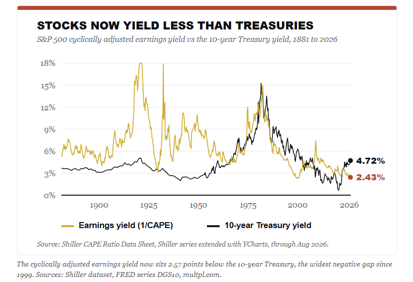
Stocks now yield 2.44% on smoothed earnings, and a 10-year Treasury pays 5.0%. That gap is the widest since 1999. For most of the previous market history, the discount rate was a tailwind, falling year after year and lifting what buyers would pay. It isn’t doing that now. And the dividend engine can’t climb back to 4.3% unless prices fall a long way first, which rather defeats the purpose.
However, there is a second channel that gets much less attention than valuations. Critically, it works through flows rather than math. From 2010 through 2020, the 3-month Treasury bill averaged 0.56%. It sat below a quarter point on 63% of all trading days. Cash paid you nothing to wait. For most of the previous decade, the entire market trade was built on the “TINA” trade. The idea that “There Is No Alternative” to risk assets was never really a thesis. It was a hostage situation. Money got pushed out of safe assets and into risk because safety had been priced at zero.
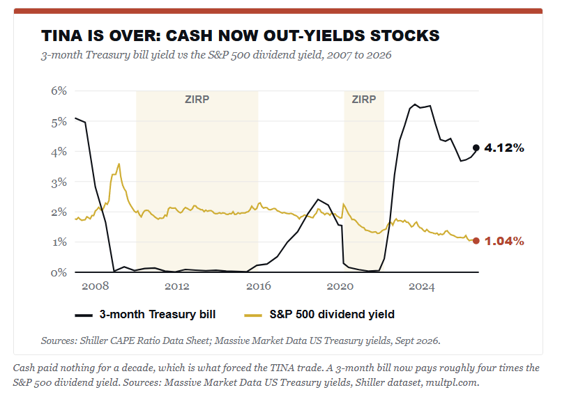
That entire scenario has now flipped with a 3-month Treasury bill paying roughly 4% today, while the S&P yields 1.06% in dividends, the lowest reading in the entire Shiller record. Cash pays roughly four times what stocks pay, with none of the drawdown risk. The same policy that once shoved money into equities can now pull it back out. That doesn’t take a forecast to matter. It just takes a retiree doing arithmetic.
I will get this comment almost as soon as this article is posted:
“You’re just repeating the mean-reversion call that’s been wrong for a decade.”
Fair enough. But I’m not making a timing call. A CAPE of 41 tells you almost nothing about next year. However, it tells you a great deal about the next ten.
What A Reasonable Investor Does With This
Start with the understanding that none of this discussion is a “forecast.” Valuations are, and always have been, a horrible timing tool. Instead, let’s examine the data in a grid. Start at a CAPE of 40.94. Add the dividend yield of 1.06%. Then vary the two things nobody can know. Where the multiple goes, and how fast real earnings grow.
FORWARD 10-YEAR REAL RETURN SCENARIOSVALUATION PATH OVER 10 YEARSREAL EARNINGS +4%REAL EARNINGS +6%CAPE stays at 415.0%7.0%CAPE drifts to 302.0%4.0%CAPE reverts to 250.2%2.2%CAPE reverts to 20-1.9%0.1%Starting CAPE 41.04, dividend yield 1.05%, as of Oct 28, 2026. Source: Shiller CAPE Ratio Data Sheet.
Those are yearly real total returns. One cell beats the last sixteen years. It also needs the most expensive market on record to stay exactly that expensive for ten more years, while earnings grow at triple their old pace. Such is the wager now priced in.
None of this argues for selling everything and waiting in cash. As I’ve written before, full market cycles have two halves, and sitting out the first half can cost you more than the second half takes. However, the grid suggests that we should calibrate our expectations. For example, if your current plan assumes a 10% nominal return because that’s the number in the brochure, you may be disappointed when your portfolio returns something nearer 3%. That gap doesn’t show up as a bad quarter. It shows up as a retirement date that moves much further out into the future.
Secondly, the hard work is both practical and dull, and you will be fighting your emotions the entire way.
Save more than the plan requires.
Trim winners back to target weights instead of letting them grow into concentration.
Own duration while it pays 5%, since the rate hurting stock valuations is the same one paying you in the bond sleeve.
And decide now what you’ll do at a 20% drawdown, because bear markets do useful work for anyone holding cash and a plan when one shows up.
Carlson is correct in his view that nobody knows what will happen next year, or the year after that. He is also right in that humility beats false precision. However, a forecast and a constraint are very different animals, and historically above-average returns from here run into the second kind. In other words, the math simply doesn’t care whether anyone believes it.
Frequently Asked Questions
What are realistic stock market returns over the next ten years?
Starting from a CAPE of 41, the arithmetic gives a range rather than a number. If multiples hold and real earnings grow 4% to 6% a year, you land somewhere around 5% to 7% in real terms. If the multiple drifts back toward 25, that falls to between 0% and 2%. None of those paths repeats the 11.41% real the market delivered over the last sixteen years.
Why were the last sixteen years so far above average?
Three engines, and they weren’t equal. Real earnings grew 4.91% a year, dividends added 1.96 points, and the valuation multiple added 4.33. Strip the multiple out and the period was unremarkable. Nearly all of those above-average returns came from investors paying more for the same dollar of smoothed profit, which is the only source that cannot be repeated from a starting point of 41.
Does a high CAPE ratio mean I should sell stocks?
No. A CAPE of 41 tells you almost nothing about next year and a great deal about the next decade. Selling on valuation alone has been an expensive mistake for most of the last sixteen years. The useful response is calibration, not an exit. Lower the return assumption your plan runs on, save more against the gap, and decide your drawdown rules before you need them.
Has an expensive market ever delivered good returns?
Once. Of the 164 months since 1881 that began with a CAPE at or above 25, twenty-four beat the long-run average, and every one of them falls between June 2014 and August 2016. That decade caught the back half of zero rates and the AI earnings expansion, and it finished with the CAPE at 41 rather than 26. The exception required the same re-rating this article argues is finished.
What does the end of the TINA trade change?
From 2010 through 2020, the 3-month Treasury bill averaged 0.56% and sat below a quarter point on 63% of trading days. Cash paid nothing to wait, so savers were pushed into equities by default. A 3-month bill now pays 4.22% against a 1.05% dividend yield on the S&P 500. Safe assets compete for capital again for the first time in fifteen years.
What is the Shiller CAPE ratio measuring?
It divides the current index price by the average of the last 10 years’ inflation-adjusted earnings. The ten-year average is the point. It smooths out the boom-and-bust in profits, so you’re comparing price against a normalized earnings stream rather than against whatever the last twelve months happened to produce.
Sources & Notes
Ben Carlson, “The End of a Golden Era For Investors,” A Wealth of Common Sense, September 2026.
Primary dataset. Shiller CAPE Ratio Data Sheet, the Robert Shiller monthly S&P 500 series (price, dividends, earnings, CPI, long interest rate, real total return price, CAPE) extended with YCharts data, complete monthly from January 1871 through August 2026. Every figure in this article other than those noted below is computed from that single file.
Methodology caveat. Shiller’s price column is a monthly average of daily closes rather than a month-end close, so computed calendar-year returns run one to three points off exact figures. Anchor checks against published calendar-year total returns, stated in real terms: 1974 reconstructed at -34.21% against -34.55%, 2020 at +16.91% against +16.81%, 2024 at +21.47% against +21.51%, 2008 at -39.29% against -37.06%, 2022 at -20.14% against -23.07%. Sign agreement is reliable. The series is used here for decomposition and frequency work, not for precise return quotes.
Sample construction. The scatter holds 1,628 monthly observations from January 1881 to August 2016. It begins in 1881 because the CAPE needs ten years of prior earnings. It ends in August 2016 because each observation requires 10 years of subsequent returns, so no month after that is yet measurable. Correlation between starting CAPE and subsequent ten-year real total return is -0.49.
Overlap caveat. Ten-year windows overlap, so the 164 months at a CAPE of 25 or higher are not 164 independent events. They cluster into four episodes: 1901, 1928 through 1930, 1995 through 2007, and 2014 through 2016. The 57 months at a CAPE of 30 or higher come from only two: 1929 and 1997 through 2002. Treat the finding as four episodes, three of which ended below average.
Correction note. An earlier build of this analysis ended the sample in June 2013 because the public dataset then in use carried dividend and CPI values only through mid-2023. That cutoff excluded the June 2014 to August 2016 starting months and produced the false claim that no expensive starting month had ever delivered an above-average decade. Rebuilding on the complete series through August 2026 corrected it.
Decomposition: real total return is split into real ten-year smoothed earnings growth, the annualized change in the CAPE multiple, and the residual dividend contribution. December 2009 to August 2026 gives 4.91, 4.33, and 1.96, totaling 11.41%. The 1881 to 2026 comparison yields 1.91 + 0.55 + 4.25, for a total of 6.72%.
Short-rate history from Massive Market Data US Treasury yields, daily 2007 through September 17, 2026. The 3-month bill averaged 0.56% from 2010 to 2020 and closed below 0.25% on 63.2% of trading days during that period. Latest reading: 4.12%.
Moody’s Baa corporate bond yield of 6.32% for August 2026, FRED series BAA. Fed total assets of $6.75 trillion as of September 16, 2026, FRED series WALCL.
Forward scenario grid: real annualized total return computed as the annualized change in the CAPE multiple from 41.16, plus assumed real earnings growth, plus the 1.04% dividend yield. Calculations by RIA Advisors.



Comments
Log in or sign up to join the conversation.