Variables For An Effective Demand Limit To The Business Cycle Part 1
Noah Smith states that there is no “cycle” to the business cycle. (link) My response on twitter was, “…there can be definable limits without a cycle.”
Can we define the limit of a business cycle?
I have a model that describes what a limit to the business cycle might look like in terms of a TFUR (total factor utilization rate). (link) The TFUR is a measure of utilizing both labor and capital…
TFUR = capacity utilization*(1 – unemployment rate)
The model and its equation are…
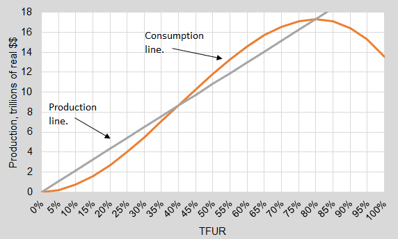
Production = PT
Effective Demand Consumption line, EDCL = PT(aT/L)(1 -(1 – 1/a)(T/L))
P = Productive capacity of the economy
T = TFUR
(PT = real GDP ouput)
L = Limit function upon T. (80% in graph) (This variable will be developed below)
a = coefficient to cross lines at L.
In the graph, the blue line is production. As utilization of labor and capital increase, production increases. The orange line represents the effective demand function to determine the consumption limit upon a business cycle. The point where the maximum of the effective-demand consumption line crosses the production line gives the natural limit of output. If production goes beyond the crossing point of the maximum, effective demand goes lower than production, which inhibits production. Production then returns to the stable equilibrium at the maximum of effective demand.
So, what variables in the economy will help us determine the effective demand limit function (L)? First let’s look at the TFUR through the decades.
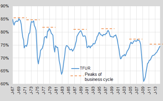
We can see cycles where the TFUR rises and then falls. I have marked the peaks of those cycles to show the limits of business cycles. These limits have been falling over the decades to lower combined utilization rates of labor and capital (TFUR). The task now is to find variables that trace a limit line on top of those business cycle peaks.
I normally use labor share to represent effective demand. (Non-farm business sector, link for data) Let’s plot the labor share index (LS) against the TFUR with the following equation…
limit function, L = LS * 0.765
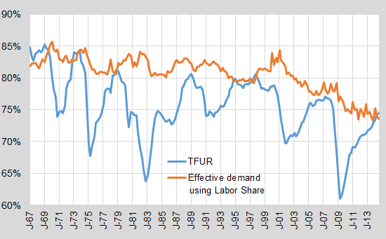
Labor share does a pretty good job at tracing the peaks, but there are some gaps at 1989 and 2005-2007. So there must be more to effective demand than just the relative domestic consumption power of labor share. What about foreign demand? Well, I can add a variable for the percentage of Net Exports to real GDP with a coefficient for the best fit to the peaks. (I keep the coefficient before of 0.765 throughout to allow the effects of other variables.)
limit function, L = (LS + 30NX/rGDP)*0.765

With foreign demand (NX/rGDP) the line still follows the descending peaks. The gap at 2005-2007 has been closed. However, the gap at 1989 is still open. Is there another variable that could close the gap at 1989 without creating other gaps at other peaks.
Let’s look at what happened in 1989. The main issue at that time was the monetary contraction of M2 and the rise in the Fed Funds rate. The Fed rate rose from 6.5% to almost 10% from March, 1988 to March, 1989. That was a strong rise. Many economists say that monetary contractions stop a business cycle expansion. So I will incorporate a measure of monetary policy to help mark a limit to a business cycle.
The variable I choose is the difference between the Fed Funds rate and my own effective demand policy rule. I subtract the Fed Funds rate from the ED rule rate (ED-FF).
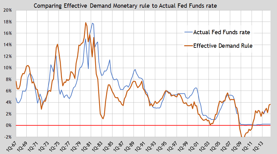
The graph shows that the Fed Funds rate rose above the ED rule in 1989. The result should have been a tightening of the limit function (L). The Fed rate also rose above the ED rule in 2000. If we incorporate the difference between the two lines in the limit function (L), will other gaps develop? Let’s find out…
I subtract the Fed rate from the ED rate such that a higher Fed rate would imply a lower limit (ED-FF). The following limit function matches the limit line to the peaks of the TFUR… (the preceding coefficients of 0.765 and 30 for NX/rGDP are kept so that the tightening of the effective demand limit by (ED-FF) can be isolated without changing LS or NX/rGDP.)
limit function, L = (LS + 30NX/rGDP + 30(ED-FF))*0.765
This equation says that if the Fed rate is set according to the ED rule based on the limit function (L) in terms of LS and NX/rGDP, production will continue to the effective demand limit. So, when the Fed rate goes higher than the ED rule, the limit function (L) based on domestic (LS) and foreign (NX/rGDP) demand will tighten possibly cutting off the business expansion prematurely. Also the model says that if the Fed rate goes lower, then the business cycle can be extended.
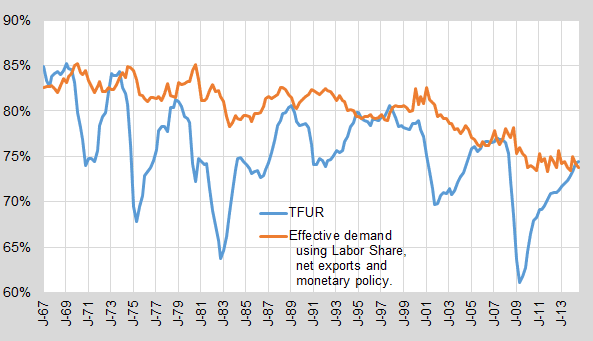
We can now see that effective demand was biting prematurely into the business expansion in 1989 due to contractionary monetary policy.
Notice that no other gaps developed as the 1989 gap closed. So it was good to include this monetary variable.
Notice also that there is a tendency for the lines to move together once they come together. This is important because it reflects the stable equilibrium of the limit model. This graph shows the stable and unstable equilibriums in the model for a limit on the business cycle.

I now put the equation for the limit function (L) into the EDCL equation. PT in the equation is replaced by data for real GDP. This is quarterly data since 1967…
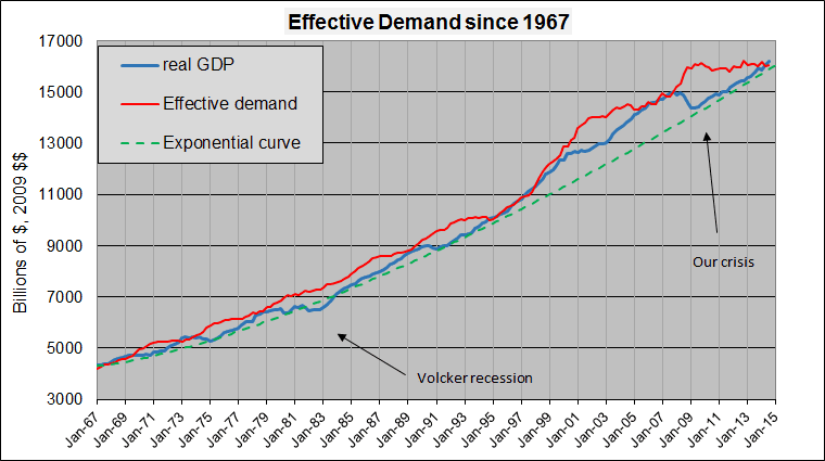
The effective demand limit stays above real GDP and shows a mostly continuous climb upwards even with occasional drops in real GDP. Since the crisis though, effective demand has been behaving differently by moving much more horizontally, which implies that productive capacity has not been increasing. When productive capacity does not rise, investment is not giving a net increase to productive capacity, but rather existing assets (speculation). The weak investment in productive capacity since the crisis is another story.
Let’s look at real GDP since 2009 plotted with the new Effective Demand limit equation (EDCL).
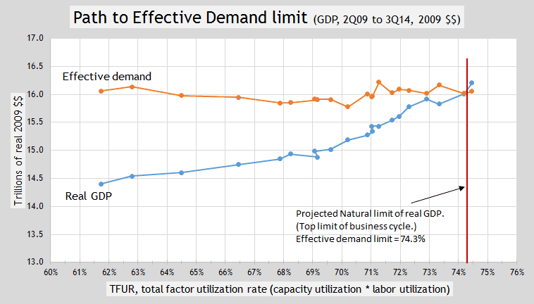
Effective demand is staying stable. (Some readers of Angry Bear should prefer this version of effective demand because there is no huge rise during a recession.)
Now the theoretical lines for consumption and production are added. Recall the equation for the Effective Demand Consumption limit…
Production = PT
Effective Demand Consumption line, EDCL = PT(aT/L)(1- (1 – 1/a)(T/L))
P = Productive capacity of the economy. P = $21.670 trillion
T = TFUR… capacity utilization*(1 – unemployment rate)
(PT = real GDP ouput)
L = Limit function using value of 74.3% based on labor share, net exports and monetary policy.
a = 3, which makes effective demand reach its limit at the limit of the business cycle.
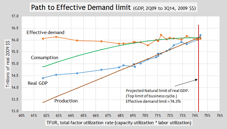
The close fit between real GDP and the production line imply that productive capacity is staying constant since the crisis. (PT only changing with changes in T, not P.)
After the dust of the crisis, the graph implies that real GDP and effective demand settled into the limit model around a TFUR of 68%.
The conclusion is that a business-cycle limit of consumption (effective demand) upon output can be modeled using variables for domestic consumption (labor share), foreign consumption (net exports/real GDP) and monetary policy (policy rule minus Fed rate). Of course, more variables can be incorporated into the limit function (L), but this lays a groundwork.
>> Continue to New Variable For Effective Demand Limit… Part 2
Disclosure: None.


