The purpose of this article is to assess the macro-fiscal flows for May 2019 and determine what effect these flows will have on the stock market and the economy.

Macro fiscal flows impact investment markets with a lagged effect of typically one month. A flush of funds now from government spending or credit creation by banks will lead to a boost in investment markets one month later.

To understand the fiscal flows, one has to look at the balance of sectoral flows within the US economy using stock flow-consistent sectoral flow analysis using the national accounts.

Professor Wynne Godley first comprehended the strategic importance of the accounting identity, which says that measured at current prices, the government's budget balance, less the current account balance, by definition is equal to the private sector balance.

GDP = Federal Spending [G] + Non-Federal spending [P] + Net Exports [X]

As a percentage of GDP, all three sectors sum to zero and balance each other out.

A table of recent sectoral balance flows is shown below:

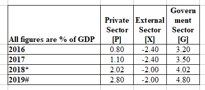
(Source: FRED plus author calculations)

*Estimate to be updated when the end-of-year numbers are known.

#Forecast based on existing flow rates and plans.

A recession has never occurred while the private domestic sector balance is in positive territory and has always happened when it is in negative territory. It is the best-kept secret national balance of accounts accounting.

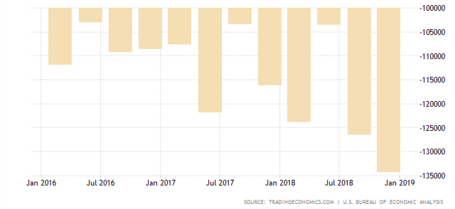
The chart below shows the newly released government budget data with the stock market superimposed over it.

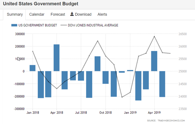
Surplus budget months are always associated with the end of a peak or a trough in the stock market.

It shows a deficit for May 2019 of $208 billion, which in reserve accounting terms means money added vertically into the economy by the currency issuer that now appears on measures of money supply, such as M1, M2, and M3. This money has been created at a keystroke as a result of the government paying its bills for goods and services received from the private sector and also for benefit payments. It is all private sector income.

The chart below shows credit creation over the same period:

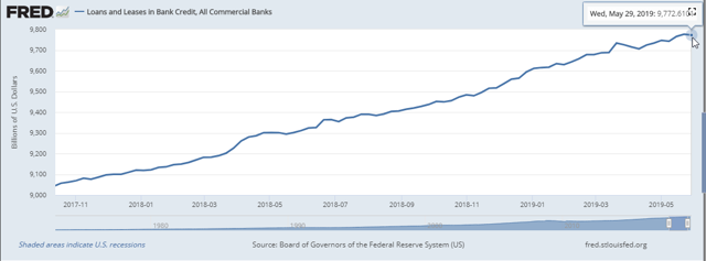
In May $25B was added to the private sector from credit creation a significant improvement from previous months where flat to negative growth had been the rule.

This adds to total credit created shown in the chart below that is reported only quarterly.

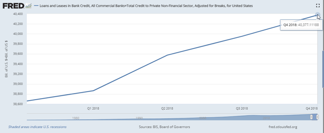
The following chart shows the current account over a similar period:

The current account gap in the United States widened to USD 134.4 billion in Q4 2018 or 2.4% of GDP. This result shows that America swapped US dollars (that it can create on a keyboard at the central bank at practically no cost) for real foreign goods and services. The stronger the dollar, the more real foreign goods and services one can have virtually for free. This is a sovereign privilege few understand.

The current account is reported quarterly, which makes the data lumpy and also outdated for analysis. A more up to date estimation of the current account position can be obtained by looking at the balance of trade, and the capital flows as these added together comprise the current account and are reported monthly.

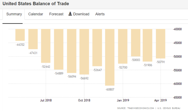
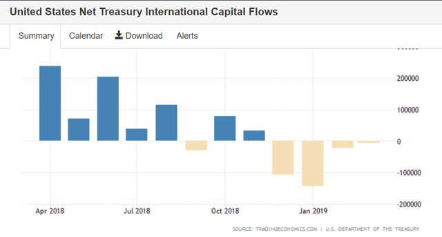
The latest balance of trade and capital flow information show that the balance of trade is steady at a deficit of around -$50B per month while the capital flows add to this deficit to produce a current account deficit of approximately $60B for the month.

Of note in the capital flows chart is the swing to a deficit and this points to less demand for the USD and one can expect the USD (USD) to fall slightly due to this lower demand, all other things equal.

Impact On Fiscal Flows

This month, the balance of account looks like this for the private domestic sector balance:

[P] = [G] + [X] is an accounting identity true by definition.

Inserting the numbers:

[P] = [$208 billion] + [-$60*]

*Estimate

[P] = $148 billion net add.

To this number, one can add the impact of credit creation [C] for May 2019 to work out the net change in the money supply and aggregate demand.

P + C = Net Money Supply Change = Domestic Aggregate Demand

$148 billion + $25 billion = $173 billion net add.

This is a positive addition to aggregate demand overall, and one can expect the market to rally into June after the dip in May caused by the large tax extraction (surplus budget) in April.

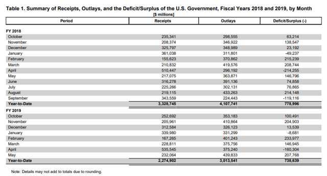
As the extract from the daily treasury statement below shows, the tax extraction was the largest ever for April at over $535B. Luckily thanks to the tax cuts the final surplus for the month was less than last year in April overall. That said the stock market still contracted and only began rising again at the start of June. Tax refunds hitting bank accounts on the 10th May found their way into the stock market approximately one month later.

The good news is that we have three good government spending input months until a bad month in September.

The Bigger Picture

The national fiscal flow pattern has to be set against the global picture. The national finances are the weather, whereas the global fiscal flows are the climate. The chart below from Mr. Robert P. Balan and his PAM service, and in this article shows the global fiscal flows on a rate of change basis.

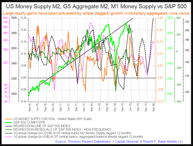
The near term macro picture is not so rosy. This peak we have just had is the best we can expect until Christmas. G5 central bank balance sheets, US and G5 M2, levels all drop from here in synchrony into September after which a Christmas rally can be expected into the new year.

There are four broad flows to watch.

1. Fedgov spending and taxation - lag one month.

2. US M2 flows - lag 6 months.

3. G5 M2 flows - lag 12 months.

4. G5 aggregate balance sheets - lag 12 months

As one can see from the chart above the four flows are all lining up for a joint decline after the short advance into summer and then will come down again in September. This is very tradable information. It is not often that the three flows synchronize like this, and when they do the results can be spectacular. One can take advantage of this information via large, broad highly liquid index funds such as SPY, DIA, QQQ and in the meantime sit out the volatility in cash (UUP) or bonds (TLT).