If you watch CNBC long enough, you are bound to hear an investment professional urging viewers to buy stocks simply because of low yields in the bond markets. While the advice may seem logical given historically low yields in the U.S. and negative yields abroad, most of these professionals fail to provide viewers with a mathematically grounded analysis of their expected returns for the equity markets.

Mean reversion is an extremely important financial concept and it is the “reversion” part that is so powerful.The simple logic behind mean reversion is that market returns over long periods will fluctuate around their historical average. If you accept that a security or market tends to revolve around its mean or a trend line over time, then periods of above normal returns must be met with periods of below normal returns.

If the professionals on CNBC understood the power of mean reversion, they would likely be more enthusiastic about locking in a 2% bond yield for the next decade. 

Expected Bond Returns

Expected return analysis is easy to calculate for bonds if one assumes a bond stays outstanding till its maturity (in other words it has no early redemption features such as a call option) and that the issuer can pay off the bond at maturity.

Let’s walk thought a simple example. Investor A and B each buy a two-year bond today priced at par with a 3% coupon and a yield to maturity of 3%. Investor A intends to hold the bond to maturity and is therefore guaranteed a 3% return. Investor B holds the bond for one year and decides to sell it because the bond’s yield fell and thus the bond’s price rose. In this case, investor B sold the bond to investor C at a price of 101. In doing so he earned a one year total return of 4%, consisting of a 3% coupon and 1% price return. Investor B’s outperformance versus the yield to maturity must be offset with investor C’s underperformance versus the yield to maturity of an equal amount. This is because investor C paid a 1% premium for the bond which must be deducted from his or her total return. In total, the aggregate performance of B and C must equal the original yield to maturity that investor A earned.

This example shows that periodic returns can exceed or fall short of the yield to maturity expected based on the price paid by each investor, but in sum all of the periodic returns will match the original yield to maturity to the penny. Replace the term yield to maturity with expected returns and you have a better understanding of mean reversion. 

Equity Expected Returns

Stocks, unlike bonds, do not feature a set of contractual cash flows, defined maturity, or a perfect method of calculating expected returns. However, the same logic that dictates varying periodic returns versus forecasted returns described above for bonds influences the return profile for equities as well.

The price of a stock is, in theory, based on a series of expected cash flows. These cash flows do not accrue directly to the shareholder, with the sole exception of dividends. Regardless, valuations for equities are based on determining the appropriate premium or discount that investors are willing to pay for a company’s theoretical future cash flows, which ultimately hinge on net earnings growth.

The earnings trend growth rate for U.S. equities has been remarkably consistent over time and well correlated to GDP growth. Because the basis for pricing stocks, earnings, is a relatively fixed constant, we can use trend analysis to understand when market returns have been over and under the long-term expected return rate.

The graph below does this for the S&P 500. The orange line is the real price (inflation adjusted) of the S&P 500, the dotted line is the polynomial trend line for the index, and the green and red bars show the difference between the index and the trend.

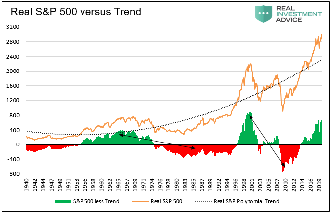
Data Courtesy Shiller/Bloomberg

The green and red bars point to a definitive pattern of over and under performance. Periods of outperformance in green are met with periods of underperformance in red in a highly cyclical pattern. Further, the red and green periods tend to mirror each other in terms of duration and performance. We use black arrows to compare how the duration of such periods and the amount of over/under performance are similar.  

If the current period of outperformance is once again offset with a period of underperformance, as we have seen over the last 80 years, than we should expect a ten year period of underperformance. If this mean reversion were to begin shortly, then expect the inflation adjusted S&P 500 to fall 600-700 points below the trend over the next ten years, meaning the real price of the S&P index could be anywhere from 1500-2300 depending on when the reversion occurs. 

We now do similar mean reversion analysis based on valuations. The graph below compares monthly periods of Cyclically Adjusted Price to Earnings (CAPE) versus the following ten-year real returns. The yellow bar represents where valuations have been over the last year.

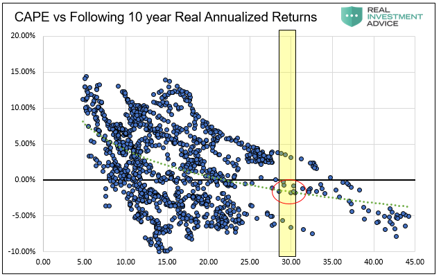
Data Courtesy Shiller/Bloomberg

Currently CAPE is near 30, or close to double the average of the last 100 years. If returns over the next ten years revert back to historic norms, than based on the green dotted regression trend line, we should expect annual returns of -2% for each of the next ten years. In other words, the analysis suggests the S&P 500 could be around 2300 in 2029. We caution however, valuations can slip well below historical means, thus producing further losses.

John Hussman, of Hussman Funds, takes a similar but more analytically rigorous approach. Instead of using a scatter plot as we did above, he plots his profit margin adjusted CAPE alongside the following twelve-year returns. In the chart below, note how closely forward twelve-year returns track his adjusted CAPE. The red circle highlights Hussman’s expected twelve-year annualized return.

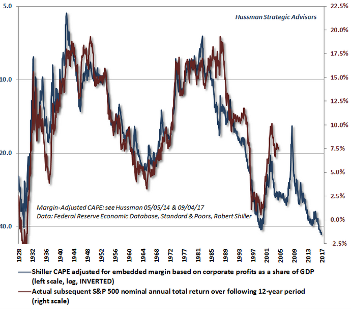
If we expect this strong correlation to continue, his analysis suggests that annual returns of about negative 2% should be expected for the next twelve years. Again, if you discount the index by 2% a year for twelve years, you produce an estimate similar to the prior two estimates formed by our own analysis.  

None of these methods are perfect, but the story they tell is eerily similar. If mean reversion occurs in price and valuations, our expectations should be for losses over the coming ten years.

Summary

As the saying goes, you can’t predict the future, but you can prepare for it. As investors, we can form expectations based on a number of factors and adjust our risk and investment thesis as we learn more.

Mean reversion promises a period of below average returns. Whether such an adjustment happens over a few months as occurred in 1987 or takes years, is debatable. It is also uncertain when that adjustment process will occur. What is not debatable is that those aware of this inevitability can be on the lookout for signs mean reversion is upon us and take appropriate action. The analysis above offers some substantial clues, as does the recent equity market return profile. In the 20 months from May 2016 to January 2018, the S&P 500 delivered annualized total returns of 21.9%. In the 20 months since January 2018, it has delivered annualized total returns of 5.5% with significantly higher volatility. That certainly does not inspire confidence in the outlook for equity market returns.

We remind you that a bond yielding 2% for the next ten years will produce a 40%+ outperformance versus a stock losing 2% for the next ten years. Low yields may be off-putting, but our expectations for returns should be greatly tempered given the outperformance of both bonds and stocks over the years past. Said differently, expect some lean years ahead.