We revisit our 10-year-old models linking real GDP per head and the rate of unemployment in developed countries. We have already validated the modified Okun’s law using new data for the USA, Canada, France, and Germany.  For the USA, we had more sources of data: the estimates from the BEA and BLS were used in addition to the OECD and Maddison Project Database. The new GDP and unemployment data covered the years between 2010 and 2019. Excellent model performance was achieved with just a few breaks in the linear link between the change rate in the GDP per capita and the change in the rate of unemployment. The years of these breaks correspond to the breaks in the GDP per head time series caused by revisions to real GDP definition.   

In this post, we apply the same approach to Australia. According to the established procedure, we first present the breaks in the GDP deflator, dGDP. The difference between the CPI and dGDP clearly reveals the definitional breaks in the dGDP estimates.  In the upper panel of Figure 1, we present the evolution of the cumulative inflation (the sum of annual inflation estimates) as defined by the CPI and dGDP between 1962 (we use the OECD data for the unemployment rate since 1961) and 2018. Both variables are normalized to their respective values in 1960. In the middle panel, the inflation rate is presented for both indices, and the lower panel displays the differences of the curves in the upper and middle panel. The difference between cumulative price change estimates has a complex structure with many pivot points. In such a complex structure, the estimated break years might be not so reliable due to larger uncertainty in the modeled parameters.

Figure 1. Upper panel: The evolution of the cumulative inflation (the sum of annual inflation estimates) as defined by the CPI and dGDP between 1961 and 2018. Both variables are normalized to their respective values in 1961.  Middle panel: The dGDP and CPI inflation estimates. Lower panel: The difference between the CPI and the dGDP curves in the upper and middle panels.

In our model, we are looking for breaks near the years and obtain the following intervals and coefficients: 

du_p = -0.76dlnG + 1.50,     1993>t≥1977

du_p = -0.35dlnG + 0.75,      2006≥t≥1993     

du_p = -0.76dlnG + 1.25,      2013≥t≥2007              

du_p = -0.36dlnG + 0.25,               t≥2014    (1)

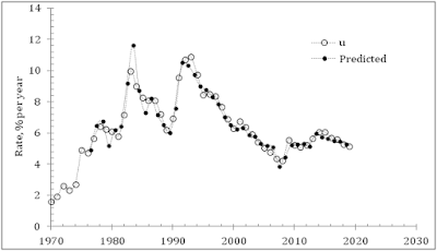
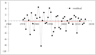
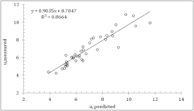
where du_p – one-year change in the (OECD) the unemployment rate , G – real GDP per capita (2011 prices). The break years are slightly different from those estimated from the inflation curves in Figure 1. This is likely due to much the higher sensitivity of the predicted unemployment rate to the coefficients in (1). As could be expected, there are 3 pivot points (breaks) in the linear dependence: 1993, 2006, and 2013. Nevertheless, the overall fit is relatively good (Rsq=0.87) as the lower panel in Figure 2 demonstrates. The revised model for Australia is successful.

Figure 2. Upper panel: The measured rate of unemployment in Australia between 1977 and 2018, and the rate predicted by model (1) with the real GDP per capita published by the MPD and the unemployment rate reported by the OECD. Middle panel: The model residual: stdev=2.5%. Lower panel: Linear regression of the measured and predicted time series. Rsq. = 0.87.