• Many investors are unnecessarily locked in an onerous bullish-bearish mindset, which severely constrains the earning power of their investment capital trapped in rigid buy-and-hold strategies.
• There's another way: trade according to the seasonality of systemic liquidity flows, especially during an era when the primary driver of risk asset prices is largess from the Fed/Treasury.
• Systemic liquidity levels create the base market conditions, but daily newsflow could dictate high-frequency moves; in the absence of compelling newsflow, the market defaults to liquidity imperatives.
• The very distinct seasonality of liquidity flows provides a basic framework for PAM's so-called "swing strategies." These basically follow the 8 major liquidity flow swings in a year, which tend to tow asset prices along their wake. Even the COVID-19 pandemic hasn't altered the tight linkage of risk asset prices to monetary flows from the Fed and Treasury.
• Setting investments long or short, depending on the seasonality of liquidity flow, plus judicious hedging and short-term trading in the direction of the liquidity seasonality flow (the "4-D Method"), unleashes the total power of compounding law. Utilizing these methods, PAM expects to deliver super-excellent 2020 year-to-date performance, now running at 1,485.92% (as of May 30).

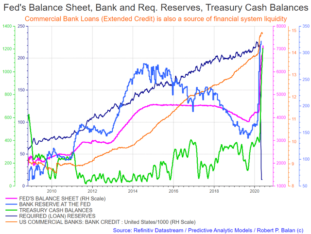
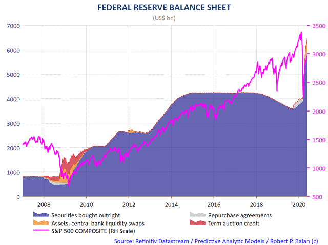
These are the primary sources of the US financial system's liquidity: The Fed's balance sheet, bank reserves (excess and required), treasury cash balances, and commercial bank loans.

(Click on image to enlarge)

 

Some definitions:

Fed's Balance Sheet - The Fed's balance sheet is a weekly report presenting a consolidated balance sheet for all 12 reserve banks that lists factors supplying reserves into the banking system and factors absorbing reserves from the system. The report is officially named Factors Affecting Reserve Balances, otherwise known as the "H.4.1" report.

Bank Reserves (Excess and Required) - bank reserves for commercial banks are held in part as a credit balance in an account for commercial banks at regional Federal Reserve banks. This credit balance used to be separated into separate "required reserves" and "excess reserves" accounts. But that distinction stopped after the Fed started to pay interest on all bank reserves. The total amount of FRB credits (bank reserves) held in all FRB accounts for all commercial banks, together with all currency and vault cash, form the M0 monetary base.

Treasury Cash Balances - The Daily Treasury Statement summarizes the US Treasury's cash and debt operations for the Federal Government on a modified cash basis. Deposits are reported as received and withdrawals are reported as processed. This account is maintained at the Federal Reserve. The US treasury pays all non-bank transactions through this account.

Commercial Bank Loans - These are the loans and leases granted by commercial banks. The deposits created as the aftermath of such loans and leases is "new money" without countervailing liabilities. These deposits are major components of M2 Money Supply.

The dynamic between these liquidity sources and risk asset prices

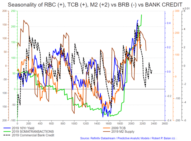
For the most part, risk assets respond mostly to changes in the Fed's Balance Sheet (RBC), the bank reserves at the Fed (BRB), and to Treasury Cash Balances (TCB). Credit creation (black, dashed line, CBC) is also important as a lead indicator of impending liquidity changes via the M2 Money Supply (brown line); see chart below.

(Click on image to enlarge)

 

Required Reserves (RRs) have been subsumed into the rubric of bank reserves, and so we do not focus on it anymore. The modeling work that we have done has been focused mainly on the Fed's balance sheet, bank reserves, and the Treasury Cash Balance. Nonetheless, RRs are a potent addition to the liquidity tool kit as a means of obtaining future TCB trends (see chart below).

(Click on image to enlarge)

 

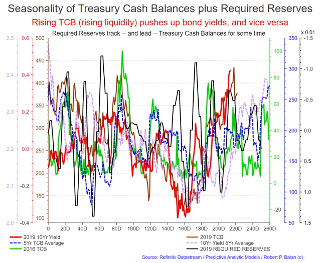
Note, in the chart above, the prevailing regime in the Fed's balance sheet, bank reserves, and TCB has been very stable since 2015. No large changes. That has been beneficial with regards to modeling because the parameters do not have to change every year since 2015.

The basic framework of the models has shown very stable seasonality among all the major sources of liquidity since 2015.

Even the COVID-19 pandemic hasn't altered the tight linkage of risk asset prices to monetary flows from the Fed and Treasury, and Commercial Banks' credit creation, as illustrated by the chart below.

(Click on image to enlarge)

 

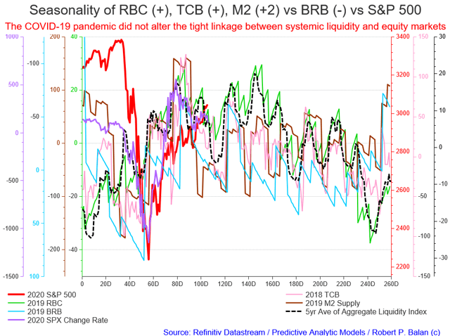
The stability and tight linkage of risk asset prices to the seasonality of systemic liquidity have enabled us to predict with success that there will be no "Sell In May" event, and that risk assets will be surging through to a peak in late May-early June. We expected a "Sell In June" phenom and a "Buy in July" event. We discussed these projections in detail in this recent article.

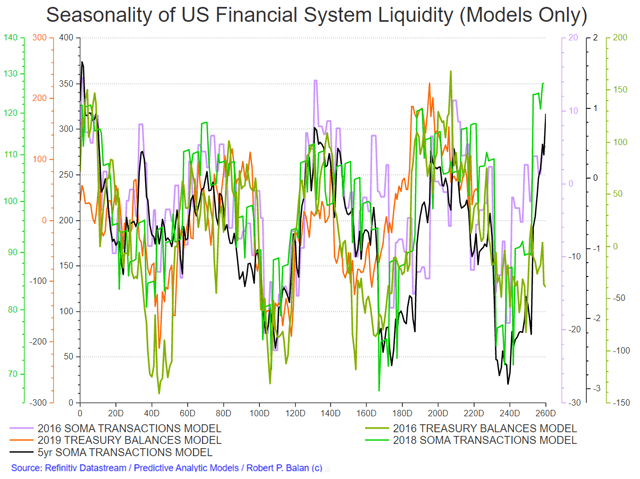
This is how the basic framework looks like every year since 2015.

This is the Basic Framework:

(Click on image to enlarge)

 

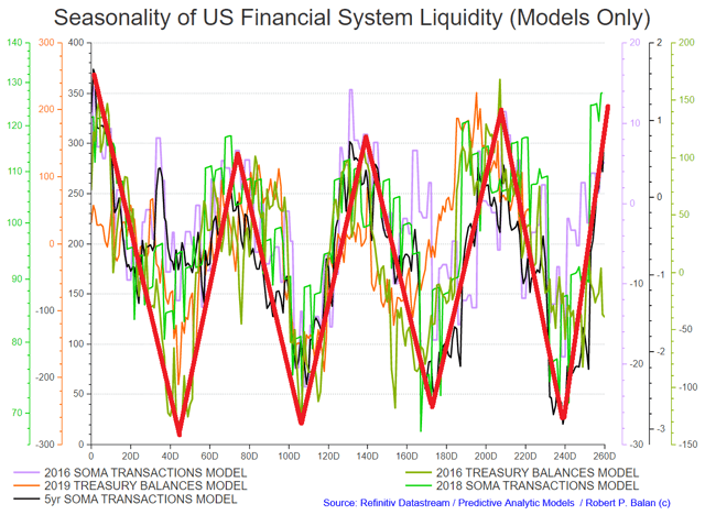
The very distinct seasonality of liquidity flows provides a basic framework for PAM's so-called "swing strategies." These basically follow the 8 major liquidity flow swings in a year, which tend to tow asset prices along their wake see chart below).

"Tactical (Swing) Strategies" from systemic liquidity framework

(Click on image to enlarge)

 

How did the risk assets perform vs. the stylized price profiles provided by the models?

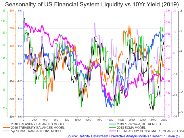
We start with bond yields and show how the 10yr yield has performed vs. the stylized liquidity flows over the past few years.

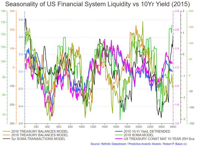
This is how 10Yr Yields performed against the Liquidity Models every year since 2015:

2020 10yr Yield vs. Liquidity Models

(Click on image to enlarge)

 

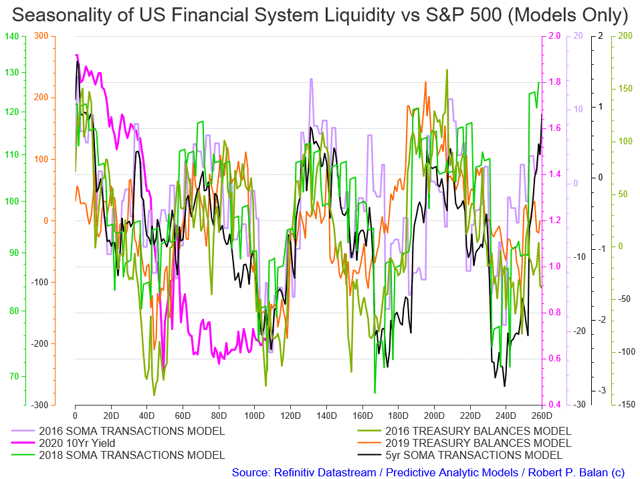
Despite the COVID-19 pandemic and the extraordinary measures taken by the Federal Reserve and US Treasury (at the direction of the Federal government), the 10y long bond yield is still hewing to the imperatives of liquidity flows.

2019 10yr Yield vs. Liquidity Models

(Click on image to enlarge)

 

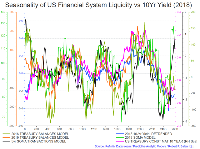
2018 10yr Yield vs. Liquidity Models

(Click on image to enlarge)

 

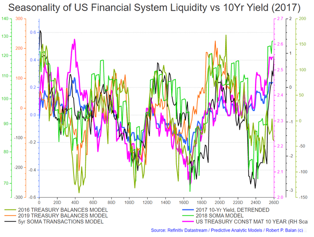
2017 10yr Yield vs. Liquidity Models

(Click on image to enlarge)

 

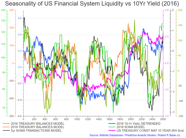
2016 10yr Yield vs. Liquidity Models

(Click on image to enlarge)

 

2015 10yr Yield vs. Liquidity Models

(Click on image to enlarge)

 

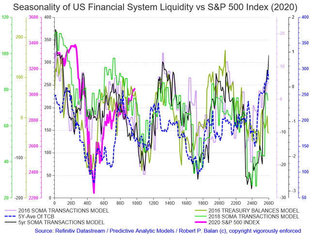
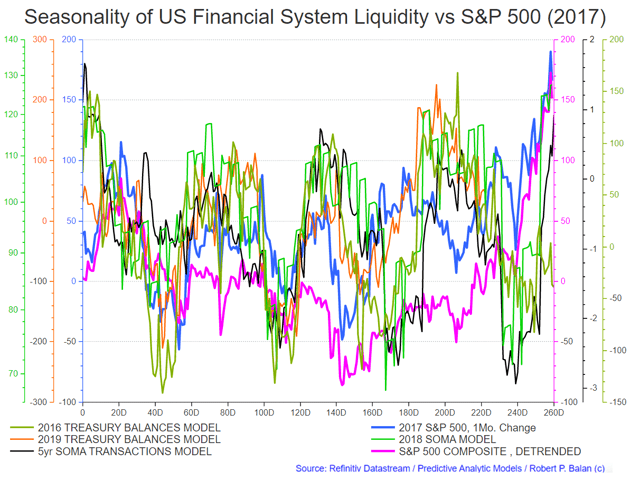
This is the performance of SPX against the models every year since 2015:

2020 SPX vs. Liquidity Models

(Click on image to enlarge)

 

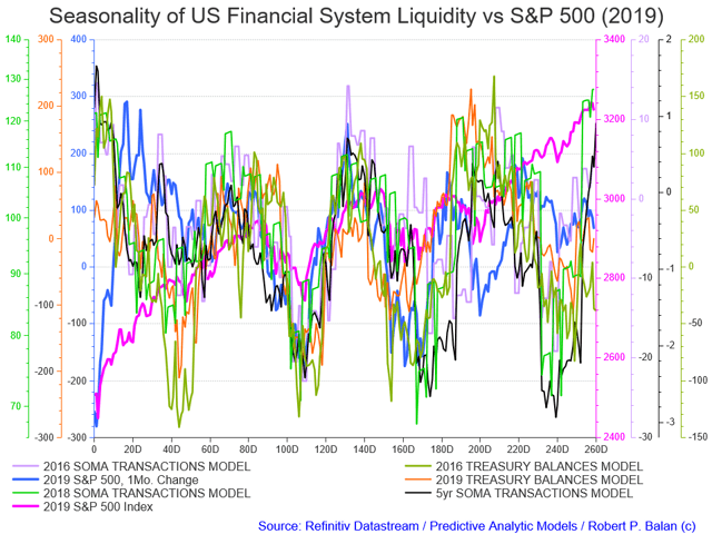
2019 SPX vs. Liquidity Models

(Click on image to enlarge)

 

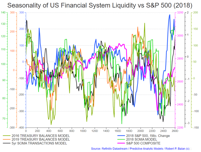
2018 SPX vs. Liquidity Models

(Click on image to enlarge)

 

2017 SPX vs. Liquidity Models

(Click on image to enlarge)

 

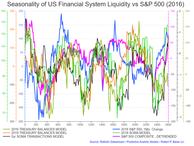
2016 SPX vs. Liquidity Models

(Click on image to enlarge)

 

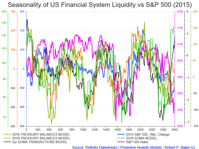
2015 SPX vs. Liquidity Models

(Click on image to enlarge)

 

Summary:

Case in point

Many investors are unnecessarily locked in an onerous bullish-bearish mindset, which severely constrains the earning power of their investment capital trapped in rigid buy-and-hold strategies.

There's another way: trade according to the seasonality of systemic liquidity flows, especially during an era when the primary driver of risk asset prices is largess from the Fed/Treasury (see chart below).

That "manna from heaven" is definitely being cut back by the Fed, something we at PAM noticed as early as three months ago. The tip-off point shown by our liquidity models was the period of May month-end and first week of June. As earlier pointed out, market action did not hold portent for a "sell-in-May" event but instead shifted that possibility for June. We will write the sequel for this article in a day or so.

Finally, the commercial banks are catching up to the fact of diminishing largess from the Fed/Treasury combo, and its likely deleterious effect on asset prices. This recent article from ZeroHedge says it all: "BofA: The "Weak" Inherited May... But Sell In June As Fed Bazooka Fades."

(Click on image to enlarge)

 

With the seasonality being highly directional, with a known length of duration, more than half of your analytical burden is solved. You can devote most of your time honing the tools to time your entry and exit in short-term trades. You can further improve the winning percentages by trading along the direction of the seasonality of the liquidity flows (which we do). This spreadsheet shows how PAM implemented that trading strategy with 95 trades in equity indices in 5 weeks and made $8,088,729.15 with 93 trades won and 2 lost.

The predictability of the seasonality of liquidity flows

US financial system liquidity flows are highly seasonal and tend to recur during the same date every year. As we can see from the illustrations, a large percentage of risk assets prices can be attributed to the influence of liquidity flows. The other segments of price movements very likely stem from daily news flow.

As we have explained before, systemic liquidity levels create the base market conditions, but daily newsflow could dictate high-frequency moves; nonetheless, in the absence of compelling newsflow, the market defaults to liquidity imperatives.

We can use the covariance of risk assets price with liquidity flows by noting the periods when liquidity conditions start to change. That also requires that we anticipate the investing behavior of investment banks and other large investors who are primary recipients of liquidity flows from the Fed and the US Treasury. We invest according to the seasonal trend in liquidity flows, confident in the fact that liquidity infusions to the Master of the Universe (Primary Dealers, investment banks and big Hedge Funds) or the MOTUs will find their way to the risk asset markets in due time.

That strategy is repeated 8 times in a year, swinging from buying to selling and then buying the risk assets again, following trend of the liquidity flows.

But the real key is capital compounding by using the "4-D Method"

Here is how Investopedia defines the Compounding Law:

Compounding is the process in which an asset's earnings, from either capital gains or interest, are reinvested to generate additional earnings over time. This growth, calculated using exponential functions, occurs because the investment will generate earnings from both its initial principal and the accumulated earnings from preceding periods. Compounding, therefore, differs from linear growth, where only the principal earns interest each period.

From its inception in May 2018, PAM has used the so-called "4-D Method" of trading style which is used by many proprietary traders in investment banks (myself included, in more than 40 years of trading). This trading strategy uses the Compounding Law and the Law of Large Numbers as core operating principles. The "4-D Method" has four key components:

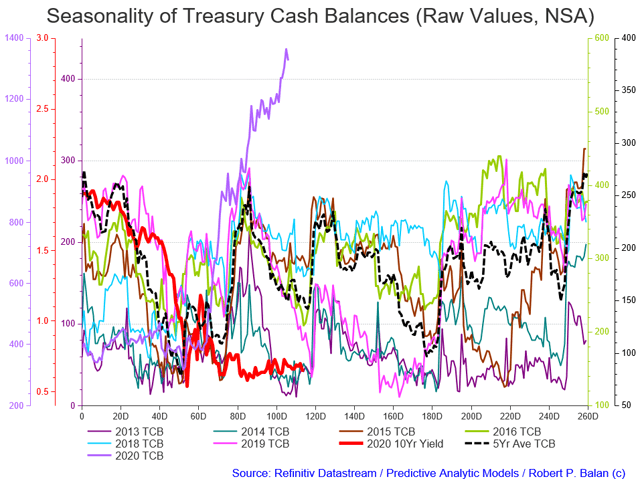
1. Trade according to the direction of the seasonality of liquidity flows. Buying risk assets (and selling bonds) when the liquidity trend is on the upswing and selling those risk assets (and buying bonds) when the seasonality flows go on the downswing. We use the Treasury Cash Balance as proxy to illustrate the predictable seasonality of aggregate systemic liquidity flows (see chart below):

(Click on image to enlarge)

 

2. Hedge errant trades, instead of using stoplosses. Trading success with a winning edge (provided by knowledge of seasonality flows and its impact on risk assets) requires a period of time for the Law of Large Numbers to take effect. You have to make a large number of individual bets for the winning edge to become inevitable and, thereby, deliver the optimal mathematical outcome.

It so happens that the Compounding Law operates on the same premise of a long process period to deliver optimal results - therefore, the larger the number of trade turn-overs happening, and the longer this process takes place, makes the inevitability of the Law of Large Numbers and the Compounding Law to become total.

But mathematical inevitability cannot take place if you lose your capital through mindless stoplosses. If you are bankrupt, there is no wherewithal for the Law of Large Numbers and the Compounding Law to make you rich.

See examples of how frequent, successful trade turnovers grow a $1 million-plus trading capital into $18 million fund valuation in five months.

See those trades here. And here.

3. We know that since liquidity seasonality makes market mean revert, hedged errant trades will become viable again because the market will eventually come close to their levels again during the next downswing in liquidity seasonality. In fact, we routinely overhedge our errant trades because we frequently make money out of the overhedged situation. In fact, our biggest single profitable trades have come from unwound overhedges.

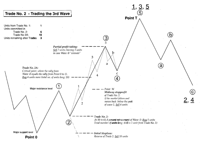
4. Implement short-term trades in the direction of the liquidity flow seasonality. We try to deploy and chop up these trades in accordance with the five-wave impulsive price action of the market as characterized by the Elliott Wave Principle (EWP) and skipping the correction phases. We deploy the most trading capital in what EWP calls as "Wave 3" when market sentiment and fundamental factors come together as a singular market narrative.

The resulting price action during this market phase tends to be the most rapid and strongest in momentum terms during the price discovery process. This provides the most substantial grist for the Law of Compounding, and so profits from these frequent successful trades build trading capital rapidly on compounded scale.

Here is how PAM implements that fourth component of the trading strategy in equities:

PAM loads to the gills with long equity futures (ES, NQ, YM, RTY) and ETFs (TQQQs, SPXLs, SPYs; which we call "Seasonals") for a seasonal run-up in liquidity. That done, we execute long scalpers (short term trades) for the initial run up from the seasonal trough.

Then we take initial profits after a satisfactory rise - those profits then serve as "trading capital" for the next set of long scalpers. If done properly, you will be playing with OPM, "other people's money", for the next set of scalpers. You have augmented your capital quickly, and on top of that, you are now financing the next set of risks from someone else's previous capital.

This initial run up is invariably followed by a "test of the bottom" - a last gasp from the bears, seeing another chance to sell on.

We reinstate the long scalpers at that bottom, in size, for a sharp impulsive run of the third wave kind (the holy grail of investment bank proprietary trading style). You may be able to do this "scalping" procedure three times in a major equity market rally.

At the top of the third, short-term trading cycle, the destination of the long scalpers and long Seasonal trades converge. What follows is pretty much is just mopping up, clearing out the scalpers and Seasonal long trades as profitable as you can time the exit.

Then we initiate short scalper trades, and when the new seasonality direction (down) is confirmed, we start accumulating seasonal short positions. And we repeat the previous process, but this time towards the downside.

This process is illustrated by a graphic from my free book, Elliott Wave Principle Applied To The Foreign Exchange Markets (which you may download here or elsewhere in the internet), see graphic below.

(Click on image to enlarge)